Table of Contents
ToggleUnderstanding Polynomial Regression
The linear regression works only when the dependent and independent variables are linearly related. But what if a simple linear line is not able to fit the linear data? In this case, we can use a polynomial line to fit the training data. This technique in machine learning is known as polynomial regression.

In this article, we will discuss in detail about polynomial-regression and its implementation in python.
What is Polynomial Regression?
Polynomial regression is a technique to use linear models to fit non-linear data. In this technique, we add additional features to the linear machine learning model. These new features are the power of existing features.
Assumptions for Polynomial Regression
As we discussed earlier, Polynomial regression is an extension of linear regression where we fit a polynomial line to the training data. Some of the assumptions for linear regression still apply to it. Here is the list of assumptions we need to follow for polynomial-regression:
Independence of errors
The errors (observed value – predicted value) are independent of each other.
Homoscadasticity
Similar to linear regression, data for Polynomial-Regression needs to be homoscedasticity. In other words, variance in residuals needs to be constant across all levels of predicted values.
Normally Distributed Prediction Error
Prediction error should follow a normal distribution with a mean equal to 0.
Data is not perfectly multi-colinear
In this, we consider that the perfect linear relation does not exists between independent variables.
Endogeneity does not exists
We need to ensure that the independent variables are exogenous. exogenous is a condition where ML model error influences the independent variables and it is opposite to endogeneity.
No Autocorrelation of Residuals
Residuals needs to be independent of each other.
Additivity
Ensure that the relationship between the independent and the dependent variable is additive. In other words, the effect of a change in one independent variable on the dependent variable is constant, regardless of the values of the other independent variables.
Why do we need Polynomial Regression
Now, question is why we need an extension of linear regression. Why linear regression can’t solve the problem. Here is the list of reasons for the requirement of polynomial regression.
- When a perfectly linear line gives high errors. Perfect linear line is not capable of fitting the training data.
- The relation between dependent and independent variables is a curve.
- We can fit more complex shapes by increasing the number of degrees of polynomials.
- Improves model performance on training and unseen data.
- A higher degree of polynomial regression becomes more sensitive to small changes in the input features.
Math Behind Polynomial Regression
Polynomial-regression fits a polynomial equation to the training data. The equation for polynomial regression is:
- Linear regression is one degree of polynomial.
- The goal of polynomial regression is to find the weights that minimize the sum of squared differences in actual and predicted values.
Cost function for Polynomial Regression
Lorem ipsum dolor sit amet, consectetur adipiscing elit. Ut elit tellus, luctus nec ullamcorper mattis, pulvinar dapibus leo.
Gradient Descent for Polynomial Regression
Lorem ipsum dolor sit amet, consectetur adipiscing elit. Ut elit tellus, luctus nec ullamcorper mattis, pulvinar dapibus leo.
Limitations of Polynomial Regression
- Highly sensitive to outliners.
- Prone to over fitting problem.
- We need to choose right polynomial degree to get a good tradeoff between bias and variance.
Linear vs Polynomial Regression
| Parameter | Linear Regression | Polynomial Regression |
|---|---|---|
| Relation between dependent and independent Variable | Linear | Non-Linear |
| Equation | ||
| Sensitivity to outliners | Less | High |
| Complexity | Low | Relatively High |
| Computation Power Requirement | Low | High |
| Feature Significance | Gives information about each feature significance. | Does not provide any information on each feature significance. |
| Over-fitting Problems | Less chances of over-fitting of data. | More prone to over-fitting of data |
Polynomial Regression implementation in Python
To implement it first we need the non-linear data with some noise. We will use numpy library.
Generate non-linear data
# Import Required Library
import numpy as np
import matplotlib.pyplot as plt
# Generate non-linear data with noise
m = 100 # Number of training examples
X = 7 * np.random.rand(m, 1) - 4
y = 2 * X**2 + 0.5*X + 4 + np.random.randn(m, 1)# Visualize the Data
plt.plot(X, y, "b.")
plt.xlabel("$x_1$", fontsize=18)
plt.ylabel("$y$", rotation=0, fontsize=15)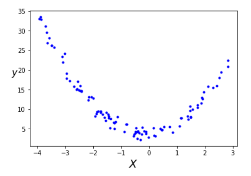
We can conclude the following points by looking at this data:
- A straight line can not fit this data.
- We need a polynomial line or curve to fit the above data points with minimum error.
Transforming data to 2nd degree of Polynomial
We will use Scikit-Learn polynomialfeature class to transform the training data. Here we will add a 2nd degree of polynomial (square of each feature) in the training set as a new feature.
from sklearn.preprocessing import PolynomialFeatures
# Add Polynomial Features
poly_feature = PolynomialFeatures(degree=2, include_bias=False)
# include_bias = True, will add a new column with all elements = 1
print ("The shape of old array X is", X.shape)
print ("The shape of new array X_poly after transformation is", X_poly.shape)The shape of old array X is (100, 1)
The shape of new array X_poly after transformation is (100, 2)
Training ML algorithm on polynomial data
# Import Linear Regression Library
from sklearn.linear_model import LinearRegression
# Training Polynomial regression model using LinearRegression Class from sklearn.linear_model library
lr = LinearRegression()
lr.fit(X_poly, y)
# Printing the weights
print("theta_0 =", lr.intercept_)
print("theta_1 and theta_2",lr.coef_) Validation of ML model on unseen data
# Create a new validation set to predic y
# Create an array of 100 numbers starting from -3 to 3.
X_new = np.linspace(-3, 3, 100)
X_new = X_new.reshape(100, 1)
y_new_actual = 2 * X_new**2 + 0.5*X_new + 4+ np.random.randn(m, 1)
print("the shape X_new data is:", X_new.shape)
# Data transformation to make predictions
X_new_poly = poly_feature.transform(X_new)
# Predicting y
y_new_predict = lr.predict(X_new_poly)plt.plot(X_new, y_new_actual, "b.", label="Actual")
plt.plot(X_new, y_new_predict, "r-", linewidth=2, label="Predictions")
plt.xlabel("$x$", fontsize=18)
plt.ylabel("$y$", rotation=0, fontsize=18)
plt.legend(loc="upper left", fontsize=14)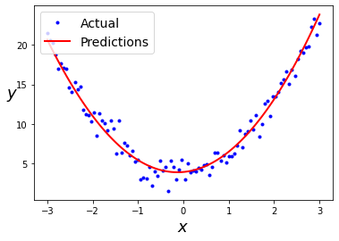
The above image shows a plot indicating predicted and actual values of dependent variable.
How to select degree of Polynomial Regression
During regression analysis, we need to ensure the best-fit line is not overfitting the training data. Over-fitting and under-fitting data in Polynomial Regression depends on the degree of polynomial. The higher the degree of polynomial, the more the chances of overfitting of data.
We can use the following techniques to solve over-fitting and under-fitting problems in polynomial regression.
- Use cross-validation to check how the model is performing on unseen data.
- Learning Curves