Analysis of Variance or ANOVA is a type of significance test in hypothesis testing where we make decisions on population based on the sample data. It is an extension of the t-test. This article covers different types of ANOVA tests, how to implement them manually, & Python language, and their applications.
Table of Contents
ToggleWhat is Analysis of Variance (ANOVA) Test
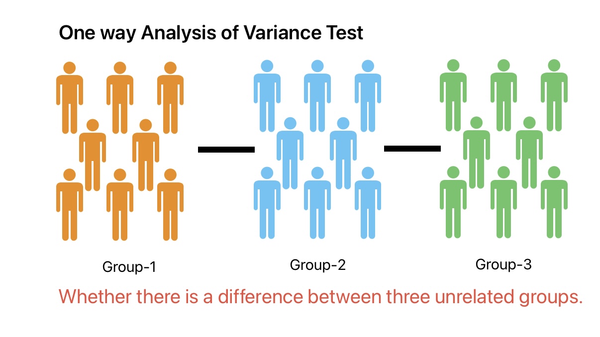
ANOVA is a statistical test in hypothesis testing to determine if there is a statistical difference between the means of three or more independent groups. It is also known as the Fisher analysis of variance.
We can use the Analysis of Variance test to determine:
- If there is a difference between three or more groups.
- Determine the influence of independent variables on the dependent variable in a regression study.
Example
- We can use ANOVA test to determine out of three machines, which machine is producing better quality products.
- Is age, profession and income have effect on the purchase decision of a product?
How ANOVA Test Works?
ANOVA test works by comparing the variability between groups with the variability within groups. The goal of the ANOVA test is to determine whether the observed difference among group means is statistically significant or it is by chance.
Formula for ANOVA Test
Mean Square (MS) = Sum of Square (SS) / Degree of Freedom (df)
Sum of Square Between Groups = Σ n ( Xj - X ) 2
Sum of Square Within = Σ ( Xij - X ) 2
- The total sum of squares measures the total variability in data and it measures the deviation of data points from their respective mean.
- Sum of squares within measures within-group variability. It gives variation within each group.
Limitations of Analysis of Variance Test
- Number of observations in each sample should be equal.
- ANOVA test assumes the variance of groups is equal. Violation of this may lead to inaccurate results.
- Data needs to be normally distributed.
- Highly sensitive to outliners.
- Does not tell which specific groups are different from each other.
- We can not use the ANOVA test with Categorical independent variables.
Assumptions for Analysis of Variance Test
We need to make sure the following assumptions for the one-way ANOVA test are met to ensure the validity and reliability of test results.
- The observations within each group should be independent of each other.
- Data is collected using random sampling
- Data within each group should be normally distributed. This assumption is not critical if the sample size is more than 30.
- All groups have an equal number of samples.
- The variances of the groups should be approximately equal.
- The dependent variable should be measured on a continuous scale.
If we violate these assumptions, it can affect the validity of the test results.
Types of Analysis of Variance Test

One-Way Analysis of Variance (ANOVA) Test
Analysis of variance have one independent variable. It determines if all samples are same or whether there is a statistically significant difference between the means of three or more independent groups.
One-way ANOVA test only tells us whether three or more groups are different. But it does not provide any indication on which of these two groups are different. Still we can know which two groups are different by using Least Significant Difference test or ad-hoc test.
Steps in One-Way Analysis of Variance Test
We will try to understand the steps to perform the Analysis of variance test using the example of plastic part manufacturing where we need to statistically prove if the part weight manufactured using 3 different machines is similar.
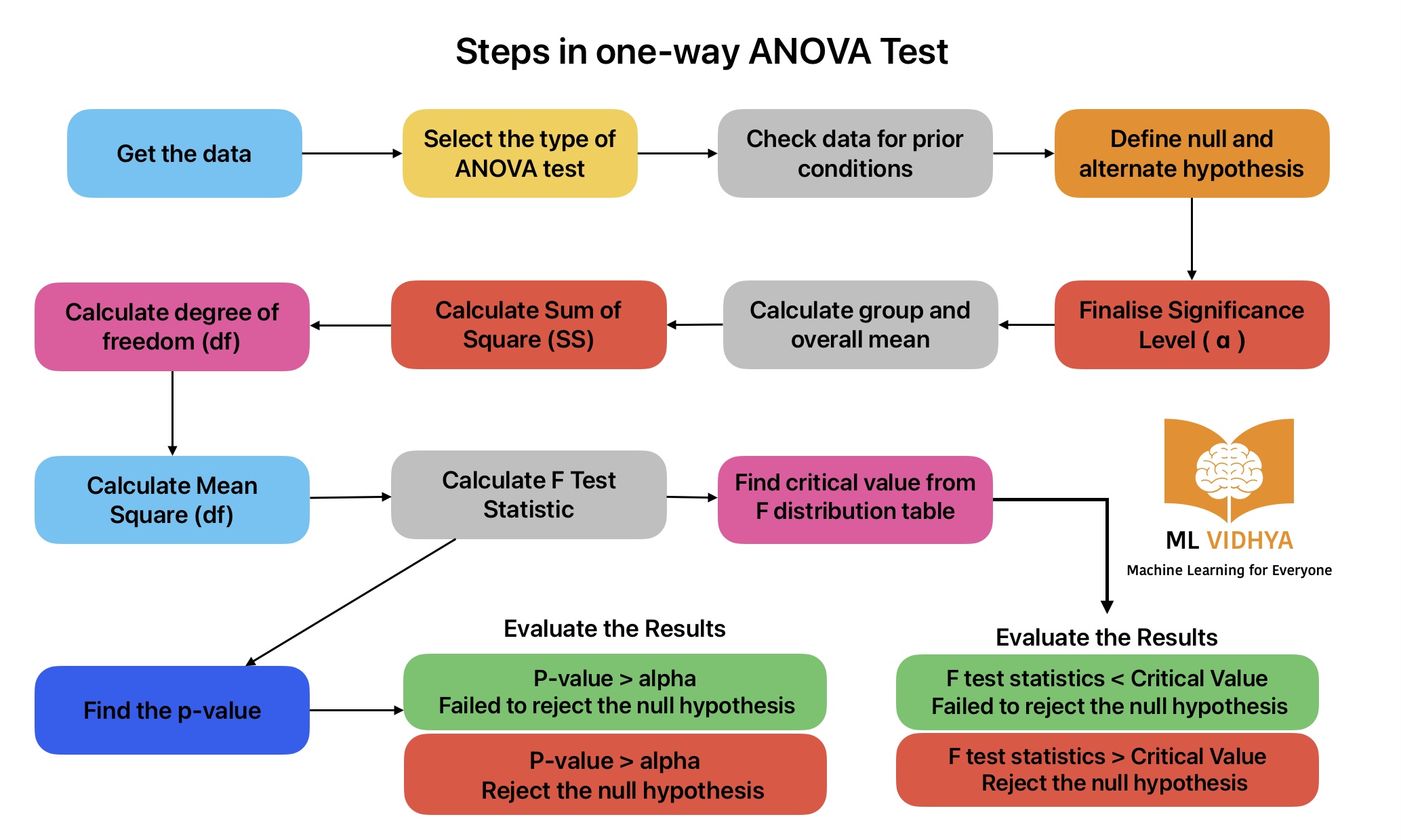
Step 1: Get the Data
| Plastic Part Weight in Grams | |||
|---|---|---|---|
| Sample Number | Machine-1 | Machine-2 | Machine-3 |
| 1 | 15 | 15.2 | 15.0 |
| 2 | 15.01 | 15.2 | 14.85 |
| 3 | 15.1 | 15.1 | 14.72 |
| 4 | 14.9 | 15.15 | 14.85 |
| 5 | 14.95 | 15.15 | 14.8 |
| 6 | 15 | 15.3 | 14.9 |
| 7 | 15.15 | 15.25 | 14.65 |
| 8 | 15 | 15.25 | 14.65 |
| 9 | 15.01 | 15.01 | 14.83 |
| 10 | 14.8 | 15.23 | 14.88 |
Step 2: Ensure data is meeting the prior conditions for ANOVA Test
Next step is to ensure data is meeting following prior conditions.
Step 3: Define Null and Alternate Hypothesis
Null Hypothesis: The mean weight of the part is equal in all parts manufactured from three different machines.
Alternative Hypothesis: The mean weight of the part is not equal from all three machines.
Step 4: Finalize the Significance Level
For this application we will consider significance level as 5% or 0.05.
Step 5: Calculate the group and overall mean
| Plastic Part Weight in Grams | |||
|---|---|---|---|
| Sample Number | Machine-1 (Group 1) |
Machine-2 (Group 2) |
Machine-3 (Group 3) |
| 1 | 15 | 15.2 | 15.0 |
| 2 | 15.01 | 15.2 | 14.85 |
| 3 | 15.1 | 15.1 | 14.72 |
| 4 | 14.9 | 15.15 | 14.85 |
| 5 | 14.95 | 15.15 | 14.8 |
| 6 | 15 | 15.3 | 14.9 |
| 7 | 15.15 | 15.25 | 14.65 |
| 8 | 15 | 15.25 | 14.65 |
| 9 | 15.01 | 15.01 | 14.83 |
| 10 | 14.8 | 15.23 | 14.88 |
| Group Mean | 14.9893 | 15.145 | 14.813 |
| Overall Mean | 14.9837 | ||
Step 6: Calculate sum of square (SS)
Sum of Square Between Groups / Treatment
SS Between Groups = 0.0003136 + 0.27324 + 0.2913 = 0.5649
Sum of square Within / Error
Xj = Mean of the group j;
SSWithin (Group-1) = 0.0846, SSWithin (group-2) = 0.08849, SSWithin(group-3) = 0.11201
SSWithin = 0.0846 + 0.08849 + 0.11201 = 0.2851
Calculate total sum of square
Step-7: Calculate the Degree of Freedom (df)
df _Treatment = k-1 = 3-1 = 2
df_error = n – k= 30-3 = 27
df_total= n-1 = 30-1 = 29
k = Total number of groups, n = Number of samples in a group
Step-8: Calculate the Mean Square (MS)
Mean Square Between Groups = 0.84159/2 = 0.420795
Mean Square Within = 0.2851/27 = 0.01056
Step-9: Calculate F-Test Statistic
F-Statistic Between Groups = 0.420795 / 0.01056 = 39.84
ANOVA Table
| Source | Sum of Squares (SS) | df | Mean Square | F |
|---|---|---|---|---|
| Between Groups (Treatment) | 0.5649 | 2 | 0.420795 | 39.84 |
| Within(Error) | 0.2851 | 27 | 0.01056 | |
| Total | 0.84159 | 29 |
Step-10: Calculate Critical F-value from F-Distribution table
For DF1 = 2, DF2 = 27, Alpha = 0.05
Critical f-value (Using F-Distribution Table) = 3.3541
Step-11: Results Evaluation
F-test Statistic = 39.84, Critical f-value = 3.3541
We can reject the null hypothesis because the F-Test statistic is greater than the critical f-value. In other words, the null hypothesis is not true, or the mean weight of the part is not equal for all three machines.
Implementation of One Way ANOVA Test in Python
We will use Python along with Scipy.stats module to perform a one-way analysis of variance. The Analysis of the variance test helps us determine if the part weight manufactured from three different machines is significantly different.
# Import Required Library in Python
import pandas as pd
from scipy.stats import f_oneway
# Create the DataFrame with from experimental data
data = {
'Machine-1': [15, 15.01, 15.1, 14.9, 14.95, 15, 15.15, 15, 15.01, 14.8],
'Machine-2': [15.2, 15.2, 15.1, 15.15, 15.15, 15.3, 15.25, 15.25, 15.01, 15.23],
'Machine-3': [15, 14.85, 14.72, 14.85, 14.8, 14.9, 14.65, 14.65, 14.83, 14.88]
}
df = pd.DataFrame(data)# Perform one-way ANOVA Test
f_statistic, p_value = f_oneway(df['Machine-1'], df['Machine-2'], df['Machine-3'])
# Print the test statistic results
print(f'F-statistic: {f_statistic:.4f}')
print(f'P-value: {p_value:.4f}')F-statistic: 35.6100
P-value: 0.0000
# Find Statistical f-value or critical f-value from f distribution table

from scipy.stats import f

# Degrees of freedom for the numerator (df_treatment) and denominator (df_error)
df1 = 2  # Number of groups - 1
df2 = 27  # Total number of observations - Number of groups

# Significance level
alpha = 0.05

# Find the critical F-value
critical_f_value = f.ppf(1 - alpha, df1, df2)

print(f'Critical F-value: {critical_f_value:.4f}')
Critical F-value: 3.3541
Result Interpretation
We can get hypothesis test results either by comparing p-value with alpha or by comparing critical f-value with test statistic.
# Results Interpretation using p-value
alpha = 0.05
if p_value < alpha:
    print('The p-value is less than the significance level. Reject the null hypothesis.')
else:
    print('Fail to reject the null hypothesis. There is not enough evidence to suggest a significant difference.')
The p-value is less than the significance level. Reject the null hypothesis.
# Results Interpretation using critical f-value
alpha = 0.05
if critical_f_value < f_statistic:
    print('Since the f-test statistic is greater than the critical f-value. Reject the null hypothesis.')
else:
    print('Fail to reject the null hypothesis. There is not enough evidence to suggest a significant difference.')
Since the f-test statistic is greater than the critical f-value. Reject the null hypothesis.
Application Examples of One-way ANOVA Test
We can use One-way Analysis of Variance (ANOVA) test to statistically compare the mean of three or more groups. Here is the list of application examples for one-way ANOVA Test:
Compare the efficiency of three different Drugs
We can compare the efficiency of three different drugs to treat a medical condition. Researcher can get the data using clinical trials.
Product Quality control in Manufacturing
We can use ANOVA test to check if the part weight manufactured from three different machines is significantly different.
Customer Feedback
Companies can get user feedback and compare product performance on three different user groups.
Machine Learning
We can use Anova test to statistically compare the mean prediction performance of three algorithms in machine learning. Based on results we can select the bes ML algorithm.
Similarly, we can apply the One-way ANOVA test in various fields such as the stock market, agriculture, Sports, and material testing to compare means across multiple groups and draw conclusions about population differences.
Two-Way Analysis of Variance (ANOVA) Test
Analysis of variance has two independent variables. For example, we can use a two-way ANOVA test to determine how two parameters (mold temperature and material temperature) impact the part manufacturing cycle time in injection molding.
In other words, we can use a two-way ANOVA test to determine if two independent variables (mold temperature and material temperature) have an impact on cycle time.
The independent variables (mold temperature and material temperature) are also known as factors and the cycle time is outcome. Here we can also split the factors into multiple levels. We can split the mold temperature as low, medium, or high.
Main and Interaction Effect in two way ANOVA Test
Two-way ANOVA test calculates a main effect and interaction effect. The main effect is similar to one-way Analysis of variance. Whereas in interaction effect, all effects are considered at the same time.
Steps in Two-Way Analysis of Variance (ANOVA) Test
We will try to understand the steps to perform the ANOVA test using an example to know the impact of experience and work function on employee salary. In other words, we will statistically check the impact of experience and work function on an employee’s salary.
For this example, we will consider factors of department and experience as A and B.
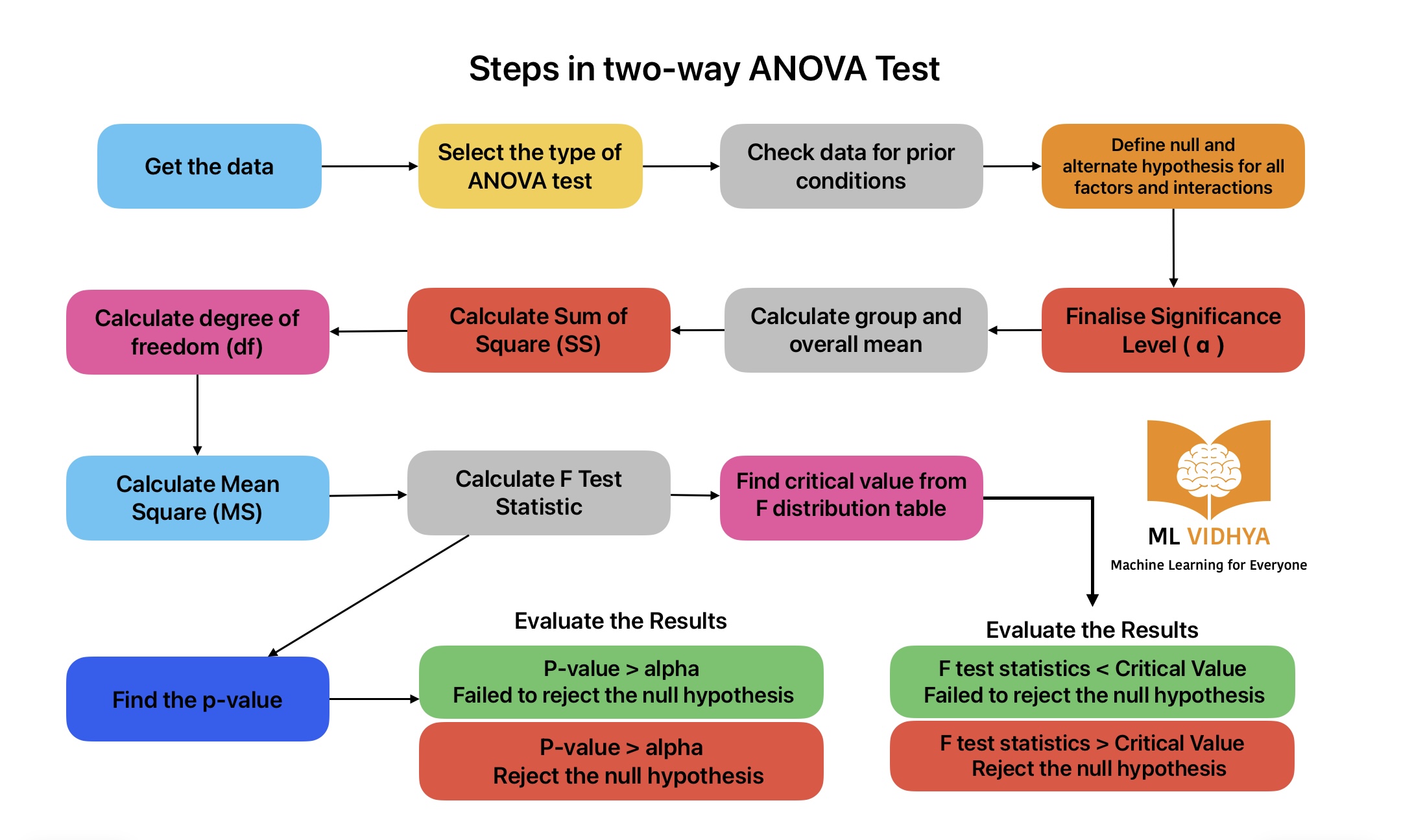
Step 1: Get the Data
| Experience (B) | ||||
|---|---|---|---|---|
| Department (A) | Fresher | Low | Medium | High |
| Software Developer | 3.5 | 6 | 10 | 20 |
| 3.6 | 8 | 12 | 15 | |
| 4.5 | 8 | 15 | 22 | |
| 4 | 5.6 | 14 | 18 | |
| Manufacturing | 2.5 | 7 | 12 | 18 |
| 3 | 7.5 | 11 | 16 | |
| 2.8 | 6 | 11.6 | 15 | |
| 3.2 | 6.2 | 13 | 17 | |
Step-2: Ensure data is meeting the prior conditions for ANOVA Test
- The population is close to normal distribution.
- All observations in data are independent.
- All groups have the same sample size.
- Population variance is equal.
Step-3: Define Null and Alternative Hypothesis
For Experience
Null Hypothesis: There is no significant difference in salary due to different levels of experience.
Alternative Hypothesis: There is a significant difference in salary due to different levels of experience.
For Department
Null Hypothesis: There is no significant difference in salary between different departments.
Alternative Hypothesis: There is a significant difference in salary between different departments.
For Interaction
Null Hypothesis: The effect of experience on salary is the same for all departments, and there is no interaction effect.
Alternative Hypothesis: The effect of experience on salary is different across at least two departments, indicating an interaction effect.
Step-4: Define Alpha or Significance Factor
For this requirement, we will consider alpha = 0.05.
Step-5: Calculate the mean
| Experience (B) | Mean | ||||
|---|---|---|---|---|---|
| Department (A) | Fresher | Low | Medium | High | |
| Software Developer | 3.5 | 6 | 10 | 20 | 10.575 |
| 3.6 | 8 | 12 | 15 | ||
| 4.5 | 8 | 15 | 22 | ||
| 4 | 5.6 | 14 | 18 | ||
| Manufacturing | 2.5 | 7 | 12 | 18 | 9.4875 |
| 3 | 7.5 | 11 | 16 | ||
| 2.8 | 6 | 11.6 | 15 | ||
| 3.2 | 6.2 | 13 | 17 | ||
| Mean | 3.3875 | 6.7875 | 12.325 | 17.625 | 10.03125 |
Step-6: Calculate the Sum of Square
Calculate the total sum of square
Calculate the Sum of Square for Factor A (Department) and B (Experience)
= 4.731+4.7358 = 9.466
SS B = 8 * ( 3.3875 - 10.03125 ) 2 + 8 * (6.7875 - 10.03125 ) 2 + 8 * (12.325 - 10.03125)2 + 8 * (17.625 - 10.03125) 2
= 940.69
Calculate the sum of square within
SS_low_experienced_Software_Developer = 4.27
SS_medium_experienced_Software_Developer = 14.75
SS_highly_experienced_Software_Developer = 26.75
SS_Fresher_production_engineer = 0.2675
SS_low_experienced_production_engineer = 1.4675
SS_medium_experienced_production_engineer = 2.21
SS_highly_experienced_production_engineer = 5
Sum of Squares within (SS within) = 0.71+4.27+14.75+26.75+0.2675+1.4675+2.21+5 = 55.425
Calculate the sum of square for interaction
SS Interaction = 4.311
Step-7: Calculate the Degree of Freedom (df)
m = total observations, j = number of levels for department=2, k = number of levels for salary=4
df_department = j-1 = 2-1 = 1
df_experience = k-1 = 4-1 = 3
df_interaction = (j-1)*(k-1) = 1*3 = 3
df_within = n – j*k = 32 – (2*4) = 24
df_total= n-1 = 32-1 = 31
Step-8: Calculate of Mean Square
MS Department = 9.466 / 1 = 9.466
MS Experience = 940.64 / 3 = 313.54
MS Interaction = -797 / 3 = -265.66
MS Within = 28.675 / 24 = 1.1947
Step-9: Calculation of F-test statistic
F-Statistic Department = 4.0624
F-Statistic Experience = 134.63
F-Statistic Interaction = 0.617
Analysis of variance Table for Two-way ANOVA Test
| Source of Variation | Sum of Squares (SS) | df | Mean Square | F-Statistic | Critical F-Value |
|---|---|---|---|---|---|
| Department | 9.466 | 1 | 9.466 | 4.0624 | 4.259 |
| Experience | 940.69 | 3 | 313.3 | 134.63 | 3.008 |
| Interaction | 4.311 | 3 | 1.437 | 0.617 | 3.008 |
| Within | 55.895 | 24 | 2.3289 | ||
| Total | 181 | 31 | 58.96 | 47.94 | 10.275 |
Step-10: Find Critical f-value from f-distribution table
Critical F-ValueDepartment = 4.259
Critical F-Value Experience =3.008
Critical F-Value Interaction =3.008
Step-11: Result Interpretation
For Department
F-test Statistic =4.0624, Critical f-value = 4.259
F-test statistic < critical F-value, we failed to reject the null hypothesis. In other words, the Null hypothesis is not True.
There is no significant difference in salary between different departments.
For Experience
F-test Statistic =134.63, Critical f-value = 3.008
F-test statistic > critical F-value, we can reject the null hypothesis. In other words, the Alternate hypothesis is True.
There is a significant difference in salary due to different levels of experience.
Combined effect of department and Experience
F-test Statistic =0.617, Critical f-value = 3.008
F-test statistic < critical F-value, we failed to reject the Null-Hypothesis. In other words null hypothesis is True.
There is a significant difference in salary due to different levels of experience.
Implementation of Two-way Analysis of Variance Test in Python
import pandas as pd
from scipy.stats import f_oneway
from statsmodels.formula.api import ols
from statsmodels.stats.anova import anova_lm

# Create a DataFrame with the provided data
data = {
    'Experience': ['Fresher', 'Low', 'Medium', 'High'] * 4 + ['Fresher', 'Low', 'Medium', 'High'] * 4,
    'Department': ['Software Developer'] * 4 * 4 + ['Manufacturing'] * 4 * 4,
    'Salary': [
        3.5, 6, 10, 20,
        3.6, 8, 12, 15,
        4.5, 8, 15, 22,
        4, 5.6, 14, 18,
        2.5, 7, 12, 18,
        3, 7.5, 11, 16,
        2.8, 6, 11.6, 15,
        3.2, 6.2, 13, 17
    ]
}

df = pd.DataFrame(data)
# Fit the two-way ANOVA model
formula = 'Salary ~ Experience + Department + Experience:Department'
model = ols(formula, df).fit()
anova_table = anova_lm(model)The above ANOVA table will output degree of freedom, sum of square, mean square, F-value and p-value.
# Print the ANOVA table
print(anova_table)
We can use following code to get F-statistic and p-value
# Extract F-statistic and p-value for Experience
f_value_experience = anova_table['F']['Experience']
p_value_experience = anova_table['PR(>F)']['Experience']

print(f"F-statistic for Experience: {f_value_experience:.4f}")
print(f"P-value for Experience: {p_value_experience:.4f}")
Application Examples of Two-way ANOVA test
We can use the two-way Analysis of Variance (ANOVA) test to compare the impact of two categorical independent variables on a continuous dependent variable. Here is the list of application examples for two-way ANOVA Test:
Compare the efficiency of two different Drugs on different genders
Determine the effect of two different drugs on patients with different genders to treat a medical condition. Researchers can get the data using clinical trials.
Product quality control in manufacturing
Evaluate the impact of two process parameters with two different machines on part rejection rate.
Marketing Research
Study the impact of different marketing strategies with different demographics on product sales.
Employee Development
Investigating the impact of two training methods and employee experience level on employee performance to do a specific task.
In Machine Learning
We can use a two-way ANOVA test in ML for the following applications.
- Evaluate the performance of different ML algorithms (Decision tree, logistic regression) and different datasets.
- Determine a machine learning model performance with different hyperparameters on different datasets.
- Evaluate the impact of different feature selection methods and preprocessing techniques on machine learning model performance.