The gradient Descent algorithm is a machine-learning algorithm that is used to train machine learning and neural network algorithms. It is one of the best available algorithms to minimize the cost function for solving machine-learning problems.
The application of the gradient descent is to find optimum values of Ө0 and Ө1 that minimize the cost function. Gradient descent minimizes the cost function by tweaking the parameters iteratively.
Table of Contents
ToggleWhat is Gradient Descent Algorithm
The gradient descent algorithm works by tweaking the parameters iteratively to minimize the cost function. Parameters that minimize the cost function are selected as final parameters.
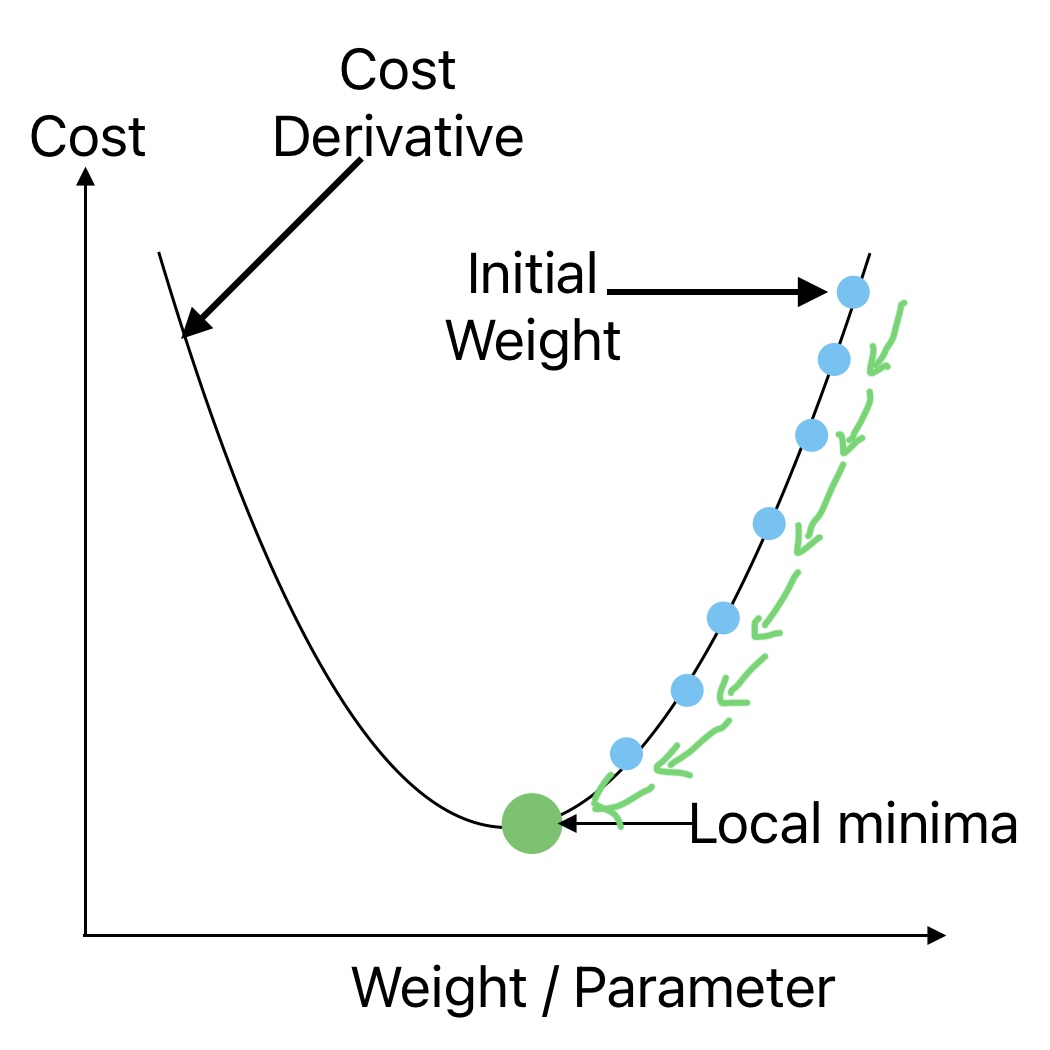
We can understand the Gradient-Decent approach using the example of a traveler on the top of a mountain. He is given the challenge to come down the mountain blindfolded.
The best strategy is to take the correct step in the correct direction where the slope is maximum. This is the only way we can reach to bottom in the shortest possible steps. The step size is critical in this approach. The gradient Descent algorithm follows a similar approach to reach the global minima where the error or cost is minimal.
Inputs for Gradient Descent Algorithm
We need the following inputs to implement gradient descent to determine the unknown parameters that minimize the cost function.
- Learning Rate or Step Size
- Random initialization parameters or weights.
- Maximum Number of Iterations
1. Impact of Leaning Rate on Gradient Decent
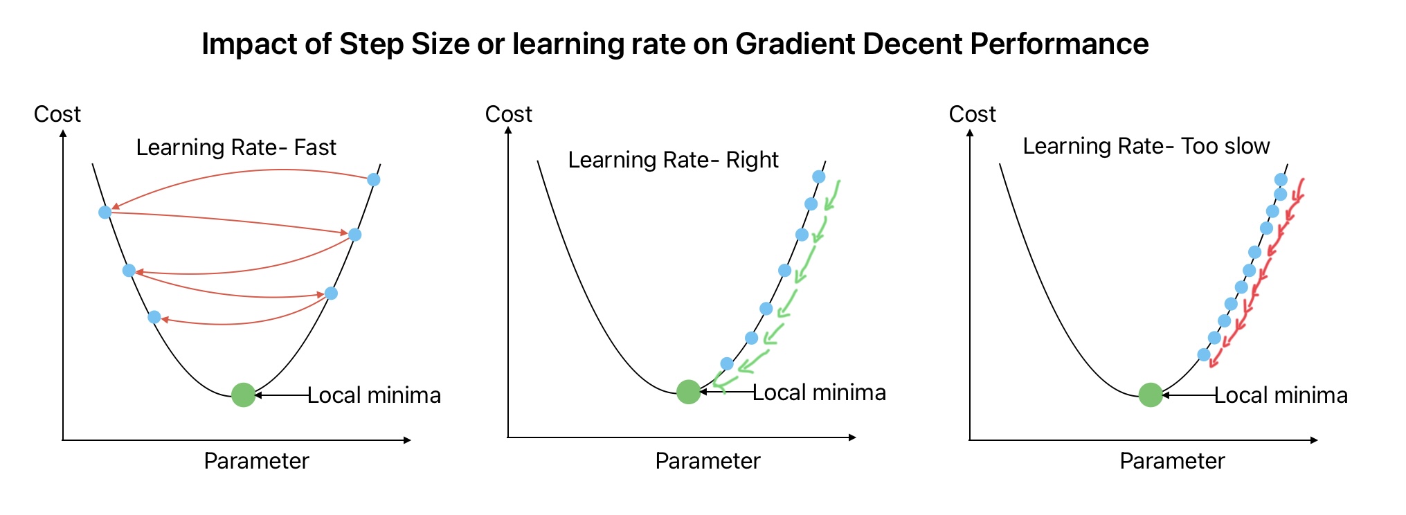
The learning rate hyper-parameter determines the step size in gradient descent algorithm implementation.
For a smaller learning rate, the algorithm will require a comparatively large number of iterations to reach global minima and converge the solution. This will increase the computational requirements and time to find the solution. For example, we need more time to come to the bottom of the hill when we take small steps.
2. Impact of Random Initialization of weights
The cost function is not always a regular bowl. It may have local minima and plateaus. These irregularities make it difficult to converge the cost function.
In gradient descent algorithm, we aim to increase the values of Ө0 and Ө1 in a direction where the squared error reduces. Apart from step size from where we start (initial values for Ө0 and Ө1) play a critical role in selecting the right parameters.
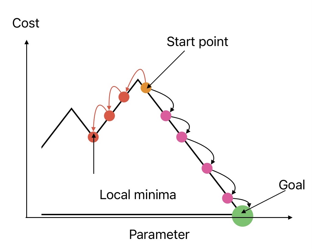
As shown in the above image, The solution will converge to local minima if the initialization starts from point A and we go towards the left side.
Whereas, the solution will converge to global minima if initialization starts from the start point and we move towards the right, provided:
- Right step size is selected.
- Solution is not stopped too early.
3. Impact of number of Iteration
We can resolve the impact of initialization (starting from left or right) just by selecting enough number of steps. The following two points ensure gradient descent algorithm reaches a global minimum provided the number of iterations is enough and the Learning rate is not large.
- For convex cost function, if we pick any two points on the curve, the line joining them never crosses the curve. As a result there are no local minima, just one global minimum.
- The cost function should be a continuous function with a slope that never changes abruptly.
Why do we need Features on the same scale for Gradient Decent
The Cost function shape is a bowl if the features are on the same scale. Whereas, it becomes an elongated bowl if the features have very different scales. With an elongated bowl, we can still get the local minima but it will take relatively more number of iterations.
Therefore it is always recommended to keep features on the same scale, otherwise, it will take longer to converge.
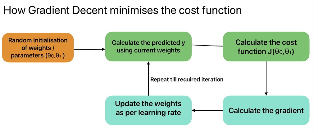
Steps in Gradient Descent to minimize cost function
Types of Gradient Descent Algorithms
We can further classify gradient descent algorithm into the following three types:
- Batch Gradient Descent Algorithm
- Stochastic Gradient Descent Algorithm
- Mini Batch Gradient Descent Algorithm
Batch Gradient Descent Algorithm
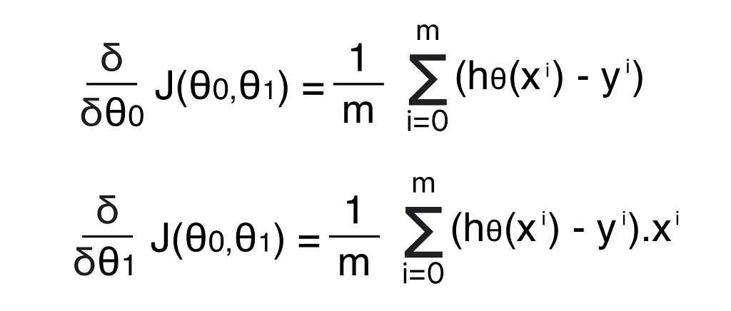
We can calculate the batch gradient descent by calculating the GD of the cost function for each parameter (Ө0 and Ө1). To calculate the gradient descent, we need to the derivative for the cost function against each parameter.
Batch gradient descent computes the gradient of the cost function over the complete batch of the training set.
Formula for Cost function for Batch Gradient Descent Algorithm
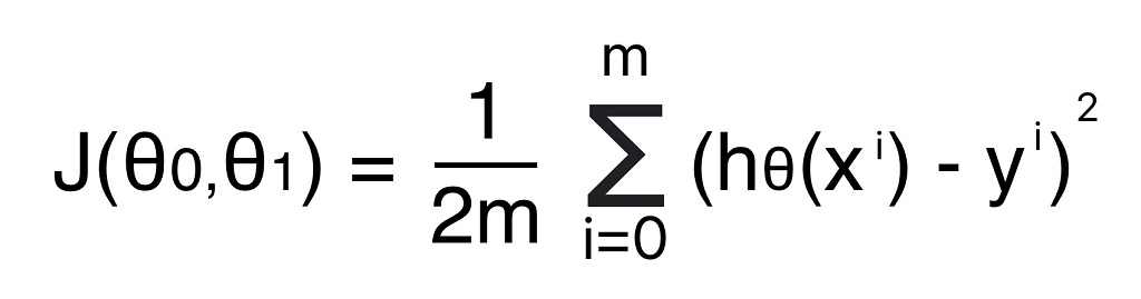
The above formula calculates the cost function over a full training set at each gradient decent step.
Formula to calculate gradient for Cost function
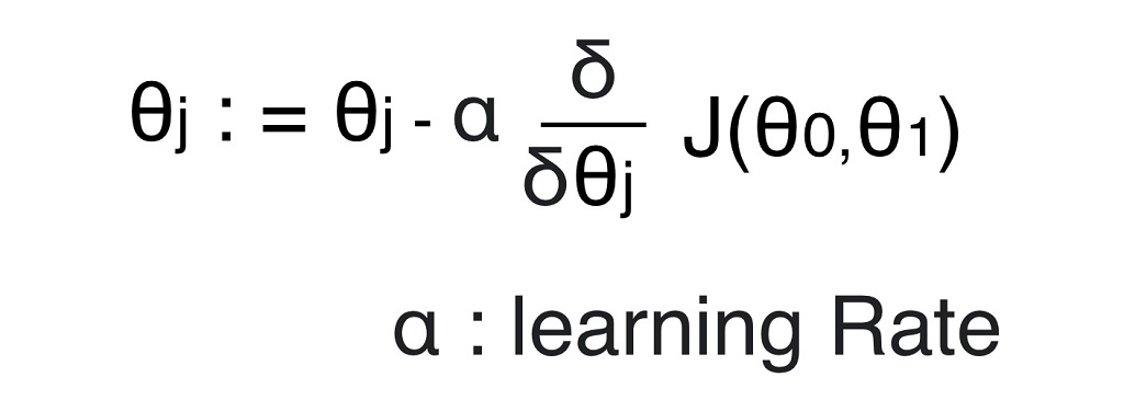
Formula to update weights as per learning rate
Implementation of Batch Gradient Descent Algorithm in Python
We can use following code to calculate the best values for weights or parameters for linear regression analysis in python.
# Defining Required Inputs for Batch Gradient Descent Algorithm

eta = 0.1  # Defining the Learning Rate
n_iterations = 1000 # Defining Maximum numbner of Iterations
m=100 # Number of data points

theta = np.random.randn (2,1) # Random Initialization of theta
print("Random initialized value for theta are:", theta)
# Running Iterations for Batch Gradient Descent
for iterations in range(n_iterations):
gradients = (2 / m)*(X_b.T).dot(X_b.dot(theta)-y)
theta = theta - eta * gradients
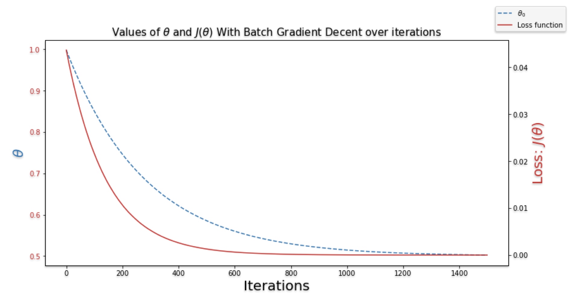
print ("The best value for theta is:", theta)Impact of Learning Rate on Batch Gradient decent Model
If the learning rate is small, it requires a lot of iterations to converge. Whereas, when the learning rate is large, It may diverge from the solution. Therefore learning rate is an important parameter that we need to optimize.
How to define the Number of Iterations for batch Gradient Descent Model
We will not get an optimum solution if you set a relatively small number of iterations. Whereas the solution time will increase drastically if we set a high number of iterations. In this case, the best approach is to:
- Set a large number of iterations.
- Interrupt the algorithm if the gradient vector becomes small.
In batch gradient descent, we take a single step or update the parameter after considering all training data. As a result, Batch GD is very slow for large training sets. In other words, Number of epochs = Number of Steps
To update the gradient descent, we take the average of the gradients of all training examples and then use a mean gradient to update the parameters.
Limitations of Batch Gradient Descent Algorithms
In batch gradient descent, the gradient is computed over the whole training dataset at each step to update the parameters. For example, if we have a million instances in the training set, the model needs to calculate one million gradients for each step. As a result, the model becomes very slow.
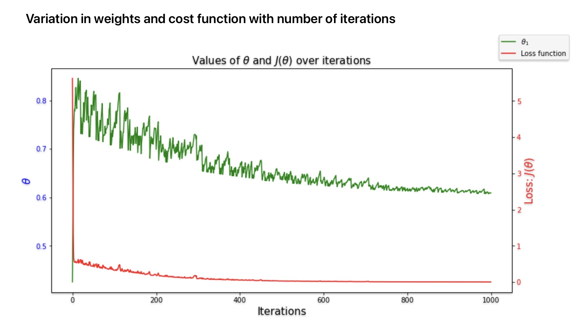
Stochastic Gradient Descent Algorithm
Instead of using all training data to calculate the gradient, Stochastic Gradient Descent uses random instances in the training data at every step. As a result, the algorithm becomes fast since it has to compute small data at every iteration.
- Reduction in the cost function is not smooth in Stochastic Gradient Decent. The cost function may increase or decrease with every iteration. But on average it always reduces with multiple iterations.
- The irregular nature of the cost function helps the algorithm skip the local minima.
Limitations or Stochastic Gradient Decent
The possibility is the SGD algorithm is not set to minima because of cost function irregular behavior. We can solve this problem by keeping the learning rate large initially and reducing it gradually as the algorithm is about to reach the solution.
- The solution can stuck in a local minimum if the learning rate is reduced quickly.
- A solution may jump around the minimum if the learning rate is reduced slowly.
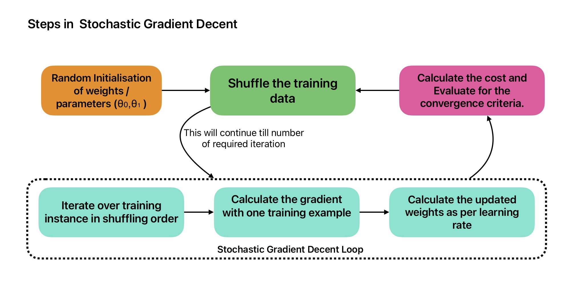
Steps in Stochastic Gradient Decent
Stochastic Gradient Descent algorithm works in the following steps:
- Pick a random instance in the training set at every step.
- Computes the gradients based only on that single instance.
- Update the weights.
Implementation of Stochastic Gradient Decent in Python
eta = 0.1  # Defining the Learning Rate
n_iterations = 1000 # Defining Maximum numbner of Iterations
m=100 # Number of data points

n_epochs = 50
# n_epochs: Number of times a learning algorithm passes through the training data
t0, t1 = 5, 50 # Learning schedule hyperparameters

# Define a function for learning schedule

def learning_schedule(t):
    return t0 / (t + t1)
theta_sgd = np.random.randn(2 , 1) # Randomization of theta
for epoch in range(n_epochs):
    for i in range(m):
        random_index = np.random.randint(m) #Generate a random number from 0 to (m-1)
        xi = X_b[random_index : random_index+1]
        yi= y[random_index : random_index+1]
        gradients = 2 * xi.T.dot(xi.dot(theta_sgd) - yi) #Calculation of gradiants
        eta = learning_schedule(epoch * m + i) #learning Rate will change wrt epoch number and sample number
        theta_sgd = theta_sgd-eta*gradients
print ("The best value for theta is:", theta_sgd)- The calculated value of unknown parameters is similar to what we calculated using batch gradient descent algorithm in relatively smaller iterations.
- In the previous case Batch Gradient Descent code iterated 1,000 times through the whole training set. Whereas, stochastic gradient descent goes through the training set only 50 times (n_epchos / m) and reaches a fairly good solution.
Implementation of SGD in Python using Scikit-Learn SGDRegressor class
We can also use Scikit-Learn SGDRegressor class to do stochastic gradient decent.
from sklearn.linear_model import SGDRegressor
sgd_reg = SGDRegressor(max_iter=1000, tol=0.05, penalty=None, eta0=0.1)
sgd_reg.fit(X, y.ravel())
print ("The best value for theta is:", sgd_reg.intercept_, sgd_reg.coef_)- The above code runs for a maximum of 1000 epochs (max_iter=1000) or until the loss drops by less than 0.05 during one epoch.
- The learning rate will start from 0.1 with the default learning schedule.
- It does not use any regularization.
Mini-batch Gradient Descent Algorithm
Mini-batch Gradient Descent takes advantage of both batch GD and Stochastic GD. It computes the gradients on small random sets of instances called mini-batches.
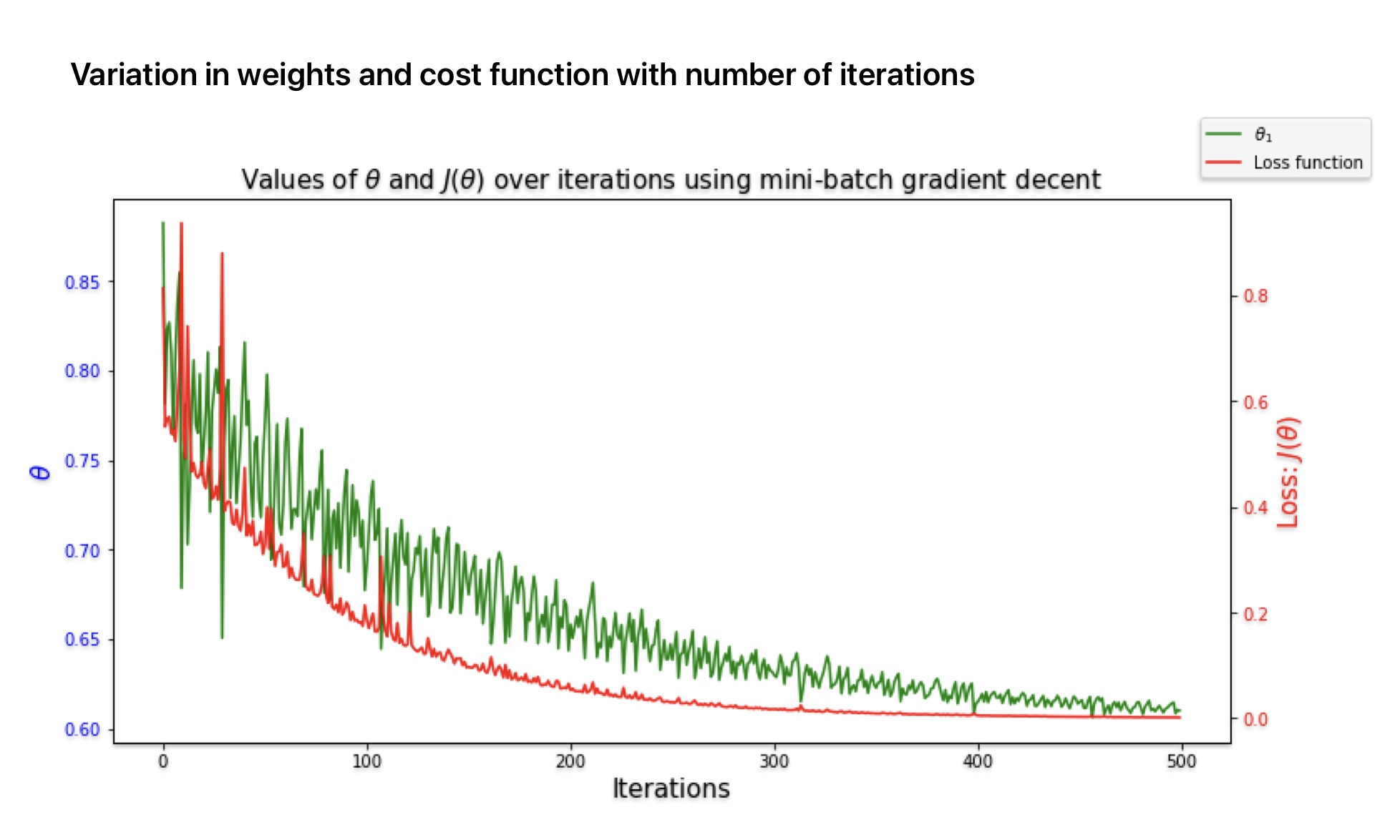
- Reduction in the cost function is comparatively less irregular in mini-batch gradient descent compared to stochastic gradient descent.
- If the batch size is large, it becomes difficult to skip the local minima.
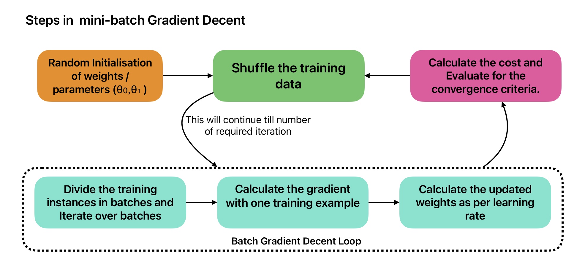
Steps in mini-batch Gradient Descent
Implementation of Stochastic Gradient Decent in Python
theta_path_mgd = []

n_iterations = 100 # Define Number of itterations
minibatch_size = 20 # Define minibatch size

np.random.seed(42)

theta_mini = np.random.randn(2, 1)  # Random initialization of theta

t0, t1 = 200, 1000  # Corrected variable names
def learning_schedule(t):
    return t0 / (t + t1)

t = 0

for epoch in range(n_iterations):
    shuffled_indices = np.random.permutation(m)
    X_b_shuffled = X_b[shuffled_indices]
    y_shuffled = y[shuffled_indices]
    for i in range(0, m, minibatch_size):
        t += 1
        xi = X_b_shuffled[i: i + minibatch_size]
        yi = y_shuffled[i: i + minibatch_size]
        gradients = 2 / minibatch_size * xi.T.dot(xi.dot(theta_mini) - yi)  # Corrected variable name
        eta = learning_schedule(t)
        theta_mini = theta_mini - eta * gradients
        theta_path_mgd.append(theta_mini.copy())  # Append a copy of theta_mini to the path

print("The best value for theta with minibatch gradient descent is:", theta_mini)
The best value for theta with minibatch gradient descent is: [[6.20309696] [1.67912157]]
Batch vs Stochastic vs Mini-Batch Gradient Descent
| Parameters | Batch GD | Stochastic GD | Mini-Batch GD |
|---|---|---|---|
| Unknown Parameters Update | Entire Training Data | One Training Instance | Batch of Training Instance |
| Update in Cost Function | Smooth: Always Decreases | Less Smooth: May increase or decrease | Irregular: May increase or decrease |
| Speed | Slow | High | In-between Batch and SGD |
| Local Minima | Difficult to skip local minima. | Irregular cost function helps the algorithm skip the local minima. | Difficult to skip the local minima for large dataset. |
| Global Minima | Reach global minima if learning rate is small and enough number of itterations are selected. | Does not guarantee convergence to the global minimum | |
Frequently Asked Questions on Gradient Descent
For a smaller learning rate, the algorithm will require a comparatively large number of iterations to reach global minima and converge the solution. whereas, with large learning rate you may skip the global minima and end up hoping around the global minima.
Best approach is to use random initialization of weights.
- Select enough number of iterations.
- The cost function is convex.
- The cost function should be a continuous function with a slope that never changes abruptly.
In batch gradient descent, the gradient is calculated using the entire training dataset. Whereas, in stochastic gradient descent, the gradient is calculated using one instance of training set.
We may end up at a sub-optimal solution and does not reach the global minimum.
Multiple Choice Questions on Gradient Descent

Time’s up