Top 10 Machine Learning Algorithms

Machine learning algorithms are computer programs that learn hidden patterns in data to provide insights. Multiple ML algorithms are available that utilize different mathematical models to generate insights or predict values from unseen data.

Today, we will get an overview of the most popular and most commonly used ML algorithms. We can broadly classify ML algorithms into the following categories.

Regression
Classification
Clustering
Association

We suggest you also read this article on Machine Learning Lifecycle to develop ML Algorithms.

Table of Contents

List of Most Common Machine Learning Algorithms

Here is the list of the most popular and commonly used algorithms:

Linear Regression
Logistic Regression
Support Vector Machines (SVM)
K-Nearest Neighbor (KNN)
Decision Tree
Ensemble Learning
Random Forest
Principal Component Analysis: PCA
K-means Clustering
XG Boost

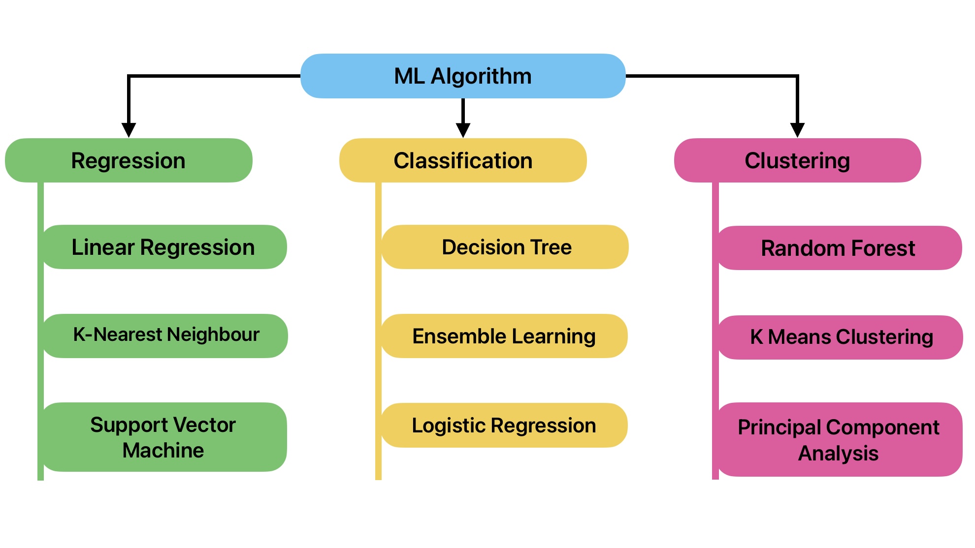
We can group these algorithms into the following three categories:

Supervised Machine Learning
Unsupervised Machine Learning
Reinforcement Learning

Linear Regression

Regression is a statistical technique to establish a relationship between the dependent (y) and the independent (X) variable. This relationship can be linear, parabolic, or something else in nature.

But in simple linear regression, the relation between dependent (y) and independent (X) variables is linear. In other words, we can define the relationship using a straight line.

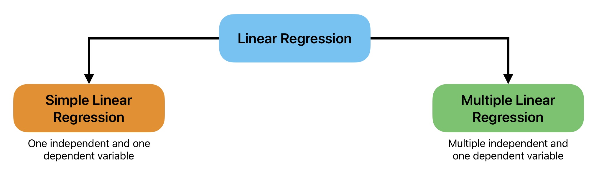
Types of Linear Regression

We can further classify Linear Regression into two types:

Simple Linear Regression
Multiple Linear Regression

Let’s consider this dataset where X is independent, and y is the dependent variable. This is a supervised machine learning problem because the output/ dependent variable is known.

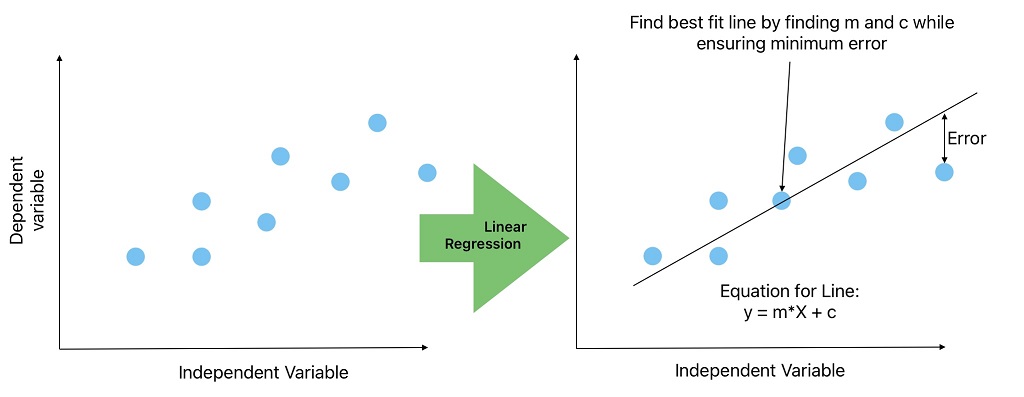
The first step in ML problem-solving is to visualize the data. When we plot a graph between the independent (X) and dependent (y) variables and find the relationship is linear. We become confident on solving this problem using simple linear regression.

In simple linear regression, we will find the best line that ensures a minimum error (Root Sum of Square, Root Mean Square) in all training data. Afterward, we can predict the unknown y values for given values of X from the best-fit line.

Equation of Line for Linear Regression

The basic equation of a simple linear regression model with one independent and one dependent variable can be represented in the following ways.

y = m X + C

y = b₀ + b₁ X

h_θ(x) = θ₀ + θ₁ X

Where:
y = Dependent Variable;
X= Independent Variable;
b₀ and b₁ or θ₀ and θ₁ are linerar Regression model parameters or weights.

In simple linear regression, we try to find the best values for m and c (constant) while ensuring minimum error. We can use the sklearn LinearRegression library for linear regression tasks.

Polynomial Regression

In some regression problems, we get complex data where a simple line cannot fit on all data points. In these cases, you can try polynomial regression to create an n-degree polynomial that fits the training data.

Polynomial regression gives a non-linear relationship between dependent and independent variables.

Equation of Line for polynomial regression

y = θ1 X + θ2 X² + c

y = dependent variable; X = independent variable, c = Constant

We can use the sklearn Linear Regression library for polynomial regression tasks.

How the polynomial model is different from the linear model?

In the linear model, we used only one independent variable X. In polynomial regression, we add more polynomial features X² as an independent variable.

We can import PolynomialFeatures from the sklearn preprocessing library to add more features.

Applications of Regression models

We can use regression algorithms for the following applications

Prepare market strategies by doing market analysis.
Evaluate returns on investments such as marketing budget vs. movie earnings.
Predicting how much a consumer is going to spend.
The relationship between two variables such as a change in resistance with temperature or, a change in water consumption with temperature.

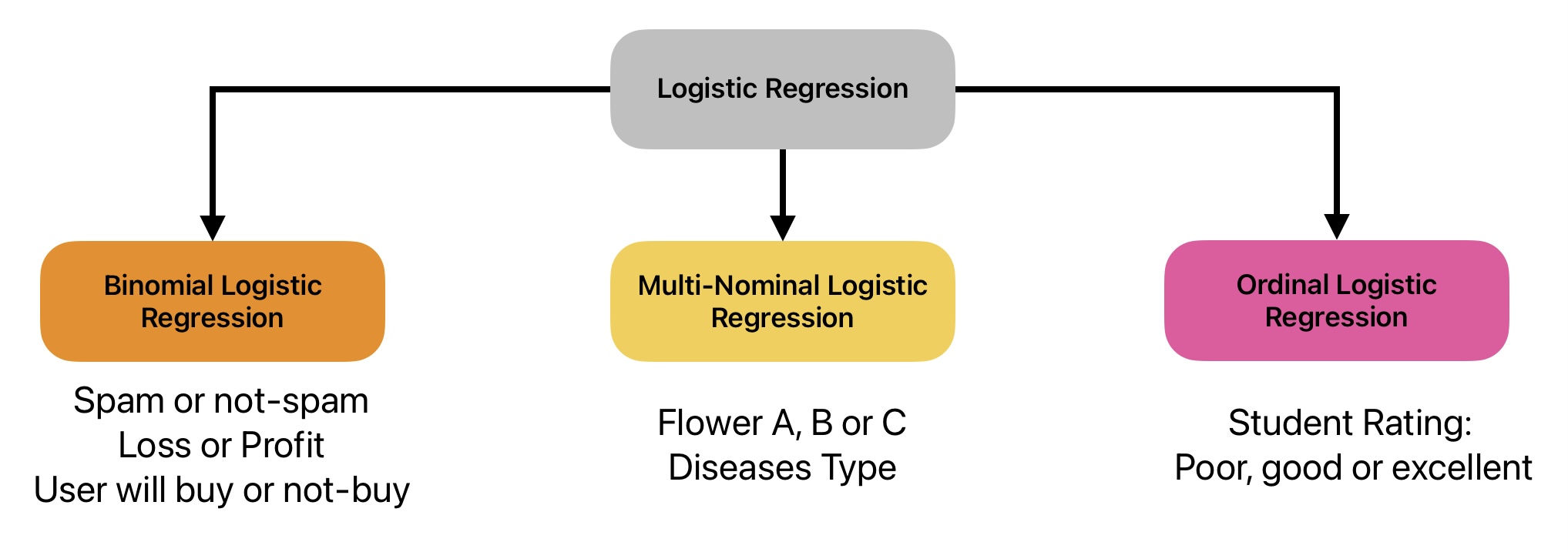
Logistic Regression

Regression models are also used for classification tasks. We can apply logistic regression where positive and negative classes are linearly separable.

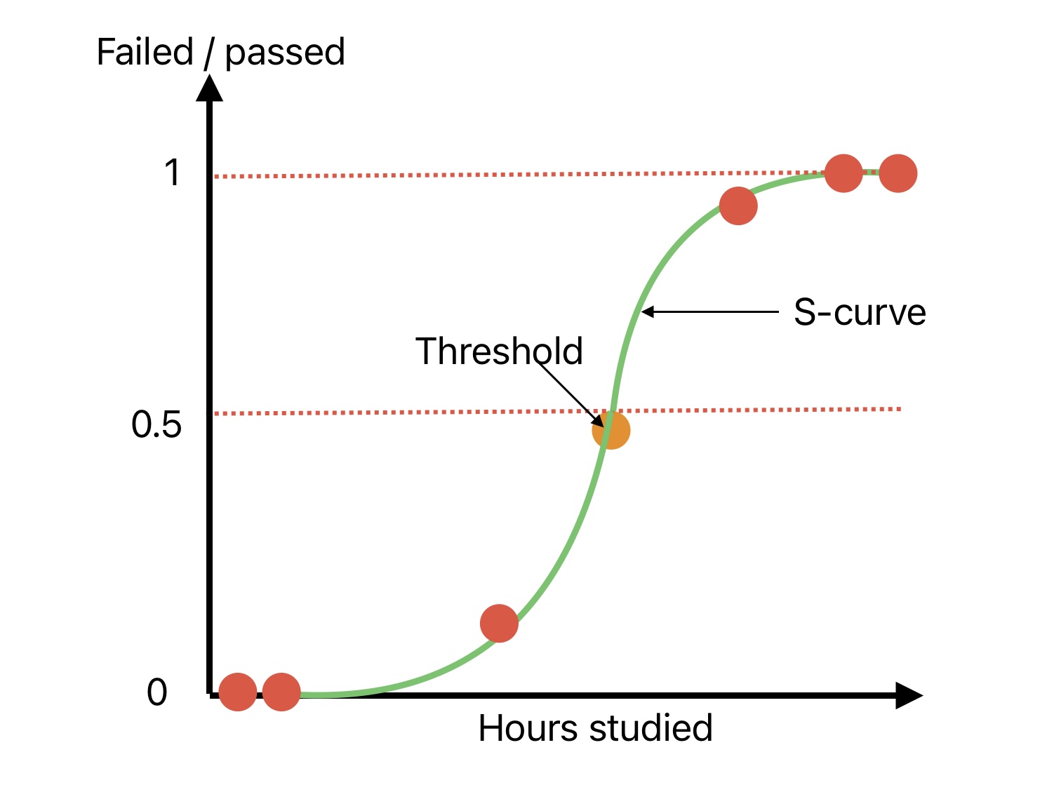
Logistic regression is a supervised ML algorithm. Its application is to estimate the probability of an instance belonging to which class. We can declare the instance class if the estimated probability of an unknown instance belonging to a particular class is greater than 50%.

Compared to linear regression, logistic regression output is between “0” to “1”. “0” being the lowest probability, whereas “1” is the highest.

Types of Logistic Regression

How does logistic regression work?

Assumption: We will denote positive points as “1” and negative points as -1. 0 is the boundary line.

Logistic regression uses a sigmoid function to ensure a large outliner does not impact the best-fit line.

Support Vector Machine

Support vector machine is a supervised ML algorithm that we can use for linear and non-linear classification, regression, and outliner detection tasks.

SVM: Machine Learning Algorithms for Classification

We can apply the SVM algorithm for classification tasks on small and medium-sized complex data sets.

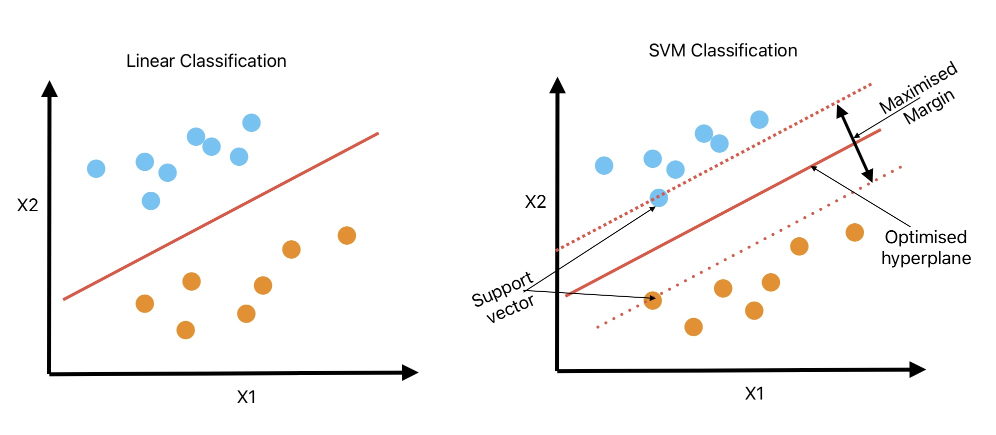
Unlike linear classification, SVM classification does not classify two classes just by linear line. SVM classifier tries to fit the widest possible street represented by two dashed lines to differentiate two classes. Therefore, SVM classifiers are also known as Margin classifiers.

We can call this path (space between two dashed lines) a street.
The SVM classifier will not be affected if we add more test points outside this street.
These two points that define the street are known as support vectors.

SVM: Machine Learning Algorithms for Regression

During the classification task, we try to get the widest possible street while ensuring there is no observation on the street.

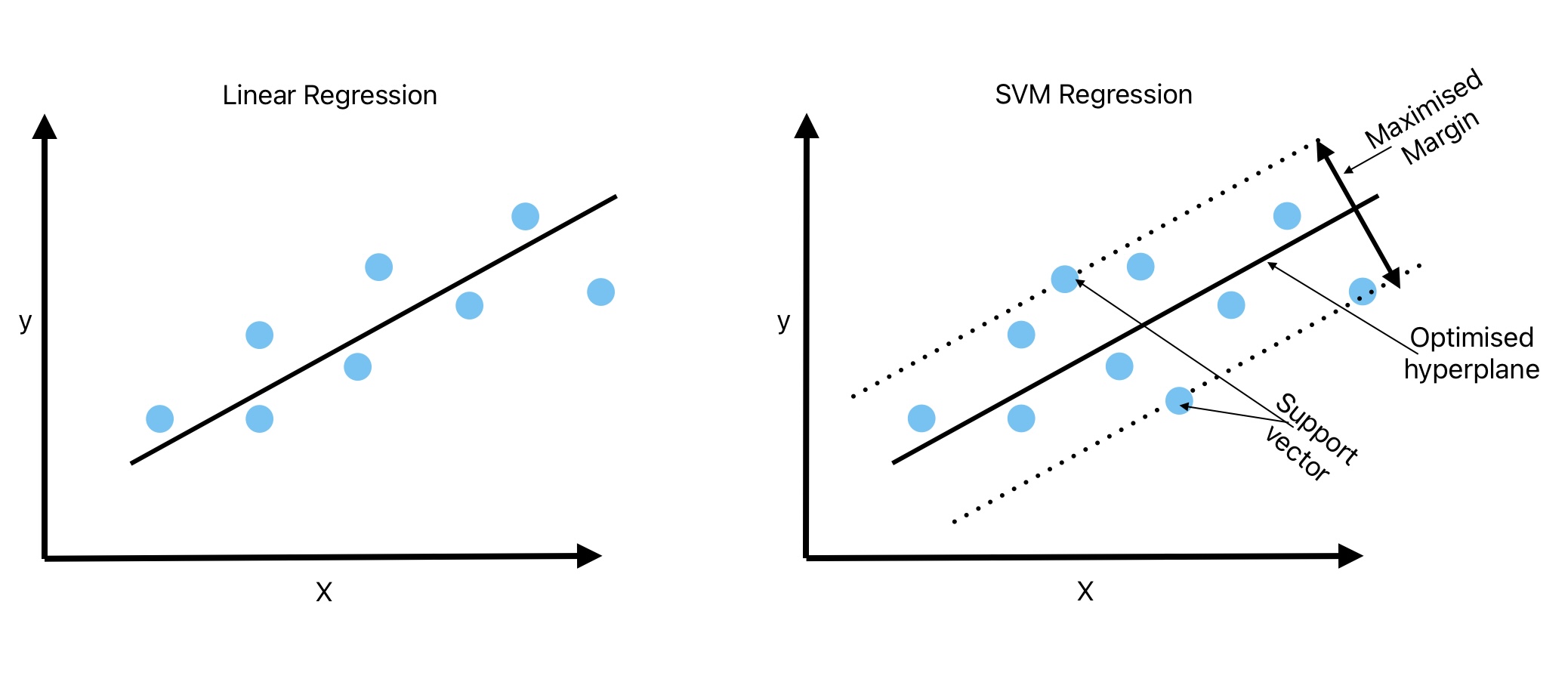
The regression task is just the opposite of classification. In SVM regression, we try to fit as many instances as possible on the street.

Applications of Support vector Machine Learning Algorithms

Here is the list of applications of SVM algorithms have applications:

Face detection
Linear and Non-Linear Regression
Linear and Non-Linear Classification
Image classification
Diseases Classification such as type of cancer
Handwriting Recognition
Intrusion Detection
Outlinear Detection

K-Nearest Neighbor (KNN)

K-nearest neighbor or KNN is a non-parametric supervised ML algorithm that we can use for classification and regression problems. Its primary application is in classification.

In KNN, we try to identify the nearest neighbor to assign a label or class to an unknown instance. We need to calculate the distance between an unknown instance and other known instances to identify the nearest neighbor.

From distance metrics, we create a decision boundary. Euclidean distance, Manhattan distance, Minkowski distance, and Hamming distance are popular distance measures in KNN.

Applications of KNN Machine Learning Algorithms

K-Nearest Neighbor has the following applications.

Data Preprocessing such as filling in the missing values
Recommendation Engine
Predicting stock prices
Predicting the risk of heart attack or cancer
Pattern Recognition.

Decision Tree

Decision trees are versatile ML algorithms that we can use for regression and classification tasks. They are also base components for Random Forest algorithms.

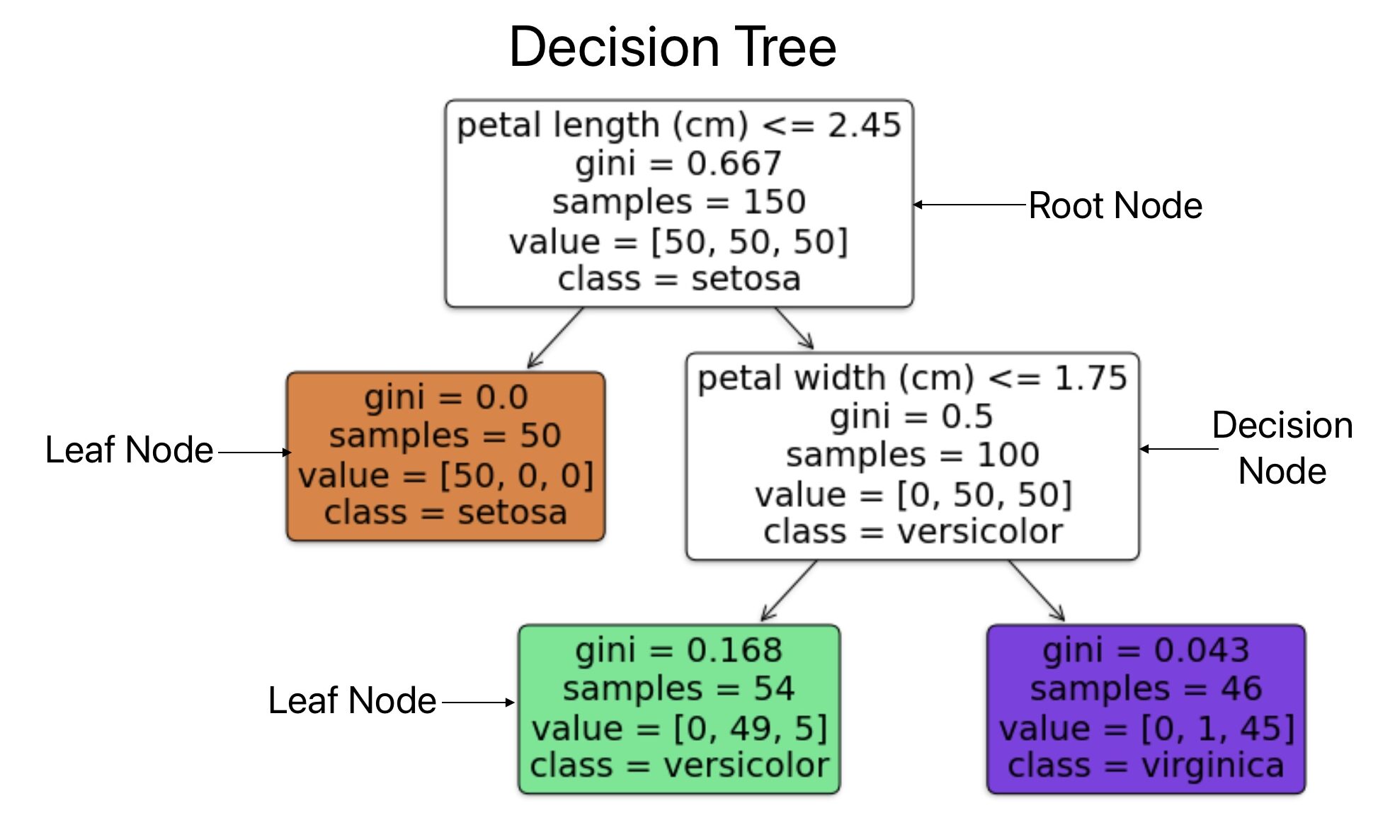
Each Decision tree consists of multiple nodes.

A decision tree starts with a root node. It is the topmost node where the decision tree starts.
The decision node is where the data branches out into possible outcomes. These outcomes give additional nodes (Decision node and Leaf node). Each decision node consists of parameters such as Condition, gini score, samples, value, and predicted class.
A leaf node is where we conclude the final decision. It does not consist of any conditions and does not ask for any questions because it makes a decision and does not ask for any questions.

Sample: Number of training instances

Value: Number of training instances from each class

Gini: It measures the impurity if the data is pure gint-0. A node is pure if all instances in a node belong to the same category.

Applications of Decision Tree: ML Algorithm

Decision trees have the following applications.

Evaluate customers with high default risk.
Customer retention by analyzing their behavior.
Preparing a marketing strategy.

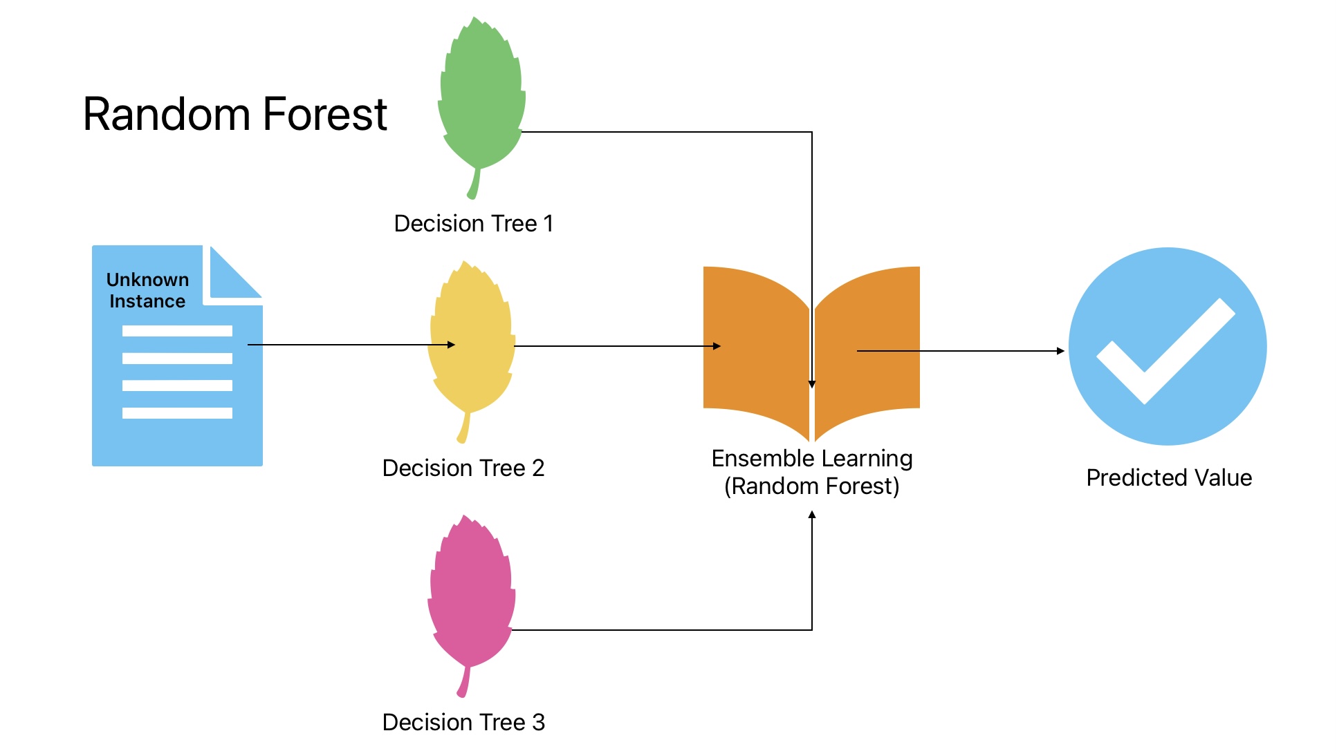
Ensemble Learning

Voting is one of the oldest techniques to make a decision. During voting, we aggregate answers from multiple people. There are chances this voting answer is better than an expert answer.

Voting classifiers are one of the popular classifiers in ensemble learning where we train multiple machine learning classifiers on the same or different data.

For any unknown input, we get the predicted value from multiple classifiers and input multiple classifier results to the voting classifier. The voting classifier aggregates the results from multiple classifiers and gives output.

Steps in Ensemble Machine Learning Algorithm

Here is the list of steps in Ensemble Learning Implementation.

Step-1: Train multiple classifiers on the training data

For example, when our goal is to classify an email: if an email is spam or not spam.

In ensemble learning, we will train multiple classifiers such as Logistic Regression, SVM classifier, Random forest, or any other classifier on the training data.

Step 2: Predict values using all trained classifiers for new unknown instances.

The next step is to predict values for unknown instances using all trained classifiers. For a particular email, if Logistic regression and random forest predict the email is spam, whereas the SVM classifier predicts it is not spam.

Step 3: Aggregating the prediction of each classifier

The next step is to aggregate the results for all classifiers ( Two classifiers are predicting the email as spam, and one classifier is predicting it as not spam). The ensemble algorithm gives output as the email is spam because the majority of votes say the email is spam.

Random Forest

Random forest is an ensemble learning technique that utilizes multiple decision trees to predict values from unknown instances. It combines the output from multiple decision trees to get one result.

Applications of Random Forest

Random Forest has applications to evaluate customers with high default risk, analyze drug responses, and make product recommendations for the e-commerce industry.

Principal Component Analysis: PCA

Sometimes, we have thousands of features for each training instance. The higher the number of features:

Slower will the training.
And getting an optimized solution becomes difficult.

PCA can reduce the number of features while keeping all information within. For example, in MNIST data, outside pixels are white in most of the images. These white pixels do not add much value during predictions. Therefore, we can drop them.

We humans can understand 2D and 3D data easily. It is very difficult to visualize data greater than 3 degree of freedom. Therefore, we can use PCA to reduce the number of features and visualize the data.

What is PCA?

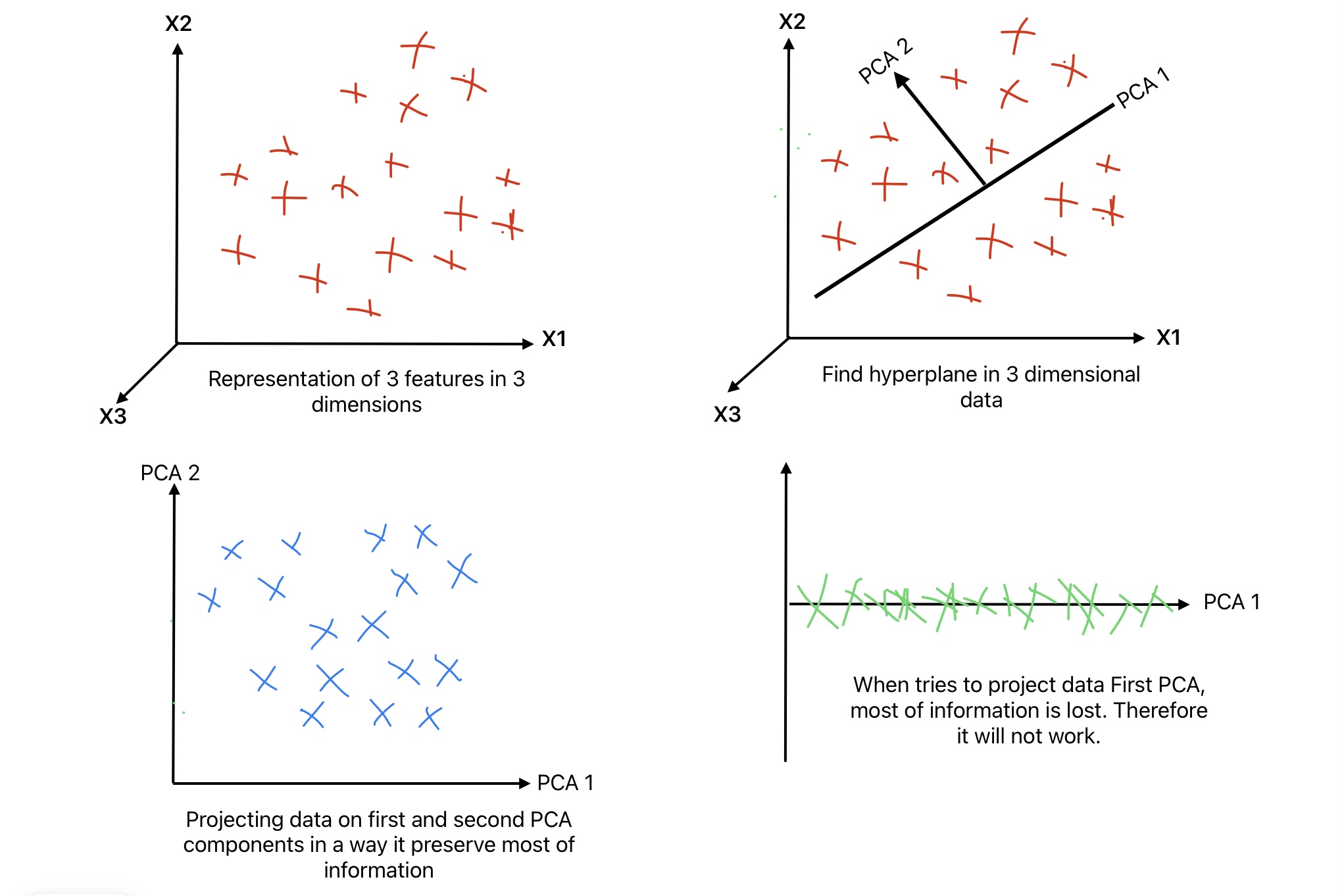
In Principal Component Analysis, we identify a hyper-plane that is close to data. Afterward, we project the data on the hyper-plane.

For example, if we have two features X1 and X2. We try to find a hyperplane that minimizes the distance. Afterward, we project the data on the hyper-plane. This new data preserves the maximum amount of variance.

K-means Clustering

K-means is an unsupervised machine-learning algorithm. Its application is to group similar items into one cluster.

It clusters the instances into one cluster ensuring the sum of the squared distance between the instance and cluster is minimal.

Example of K-means Clustering

We will consider an example of a customer where we have customer income and their spending to understand k-means clustering.

We can define customers into the following four categories.

Low-income high spending
Low-income low spending
High-income high spending
High-income low spending

Let’s try to understand how this k means clustering works.

Conclusion

Machine learning is changing the way we do business. It has applications in industries such as medical, manufacturing, hospitality, and entertainment. Multiple Machine Learning algorithms are available, and each has a different application. We need to select the best algorithm for an application. The best way is to try multiple algorithms.

We suggest you read this article on the steps in Machine learning Lifecycle.

Thanks for Reading! Enjoy Learning

Top 10 Machine Learning Algorithms