Softmax regression (Multinomial Logistic Regression or Maximum Entropy Classifier) is a technique of logistic regression to handle multiple classes. Compared to logistic regression, where we can identify two classes (0 or 1). We can use softmax regression to identify multiple classes (0, 1, 2, …., k). This article covers details on softmax regression and its implementation in Python.
Table of Contents
ToggleWhat if Softmax Regression in Machine Learning
Softmax regression ( or multi-nominal regression) combines multiple binary classifiers to classify multiple classes without the need to train multiple binary classifiers. The objective of the softmax regression classifier is to predict a high probability for true classes and a lower for false classes.
Softmax regression is an extension of logistic regression. Here is the list of key points that make it different from logistic regression
- The goal of multinomial regression is to assign a probability to all the classes in a way the total sum of probabilities is equal to 1.
- Softmax regression predicts only one class (class with maximum probability) at a time. In other words, we cannot use this to classify multiple people in a picture.
- Multinomial regression in data science uses an extension of the sigmoid function ( also known as the softmax activation function) to convert continuous values into probabilities.
- We will use cross-entropy loss as the cost function.
- We can use gradient descent for training the Softmax regression in machine learning.
How Softmax Regression works?
Softmax regression estimates the probability of an instance belonging to a given class by using the softmax function. The softmax score is an input to the softmax function. The first step in the implementation of softmax regression is to calculate the softmax score for an instance for each class.
Softmax function computes the exponential of every score, then normalizes them (dividing by the sum of all the exponentials). Similar to the Logistic Regression classifier, the Softmax Regression classifier predicts the class with the highest estimated probability.
Calculation of Softmax Score for class k
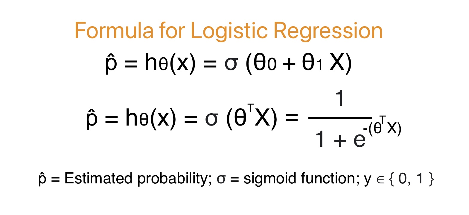
To understand softmax regression score, firstly we need to understand logistic regression.
Compared to logistic regression that output a single probability value for positive class value. The softmax regression outputs a vector that gives a probability of each class.
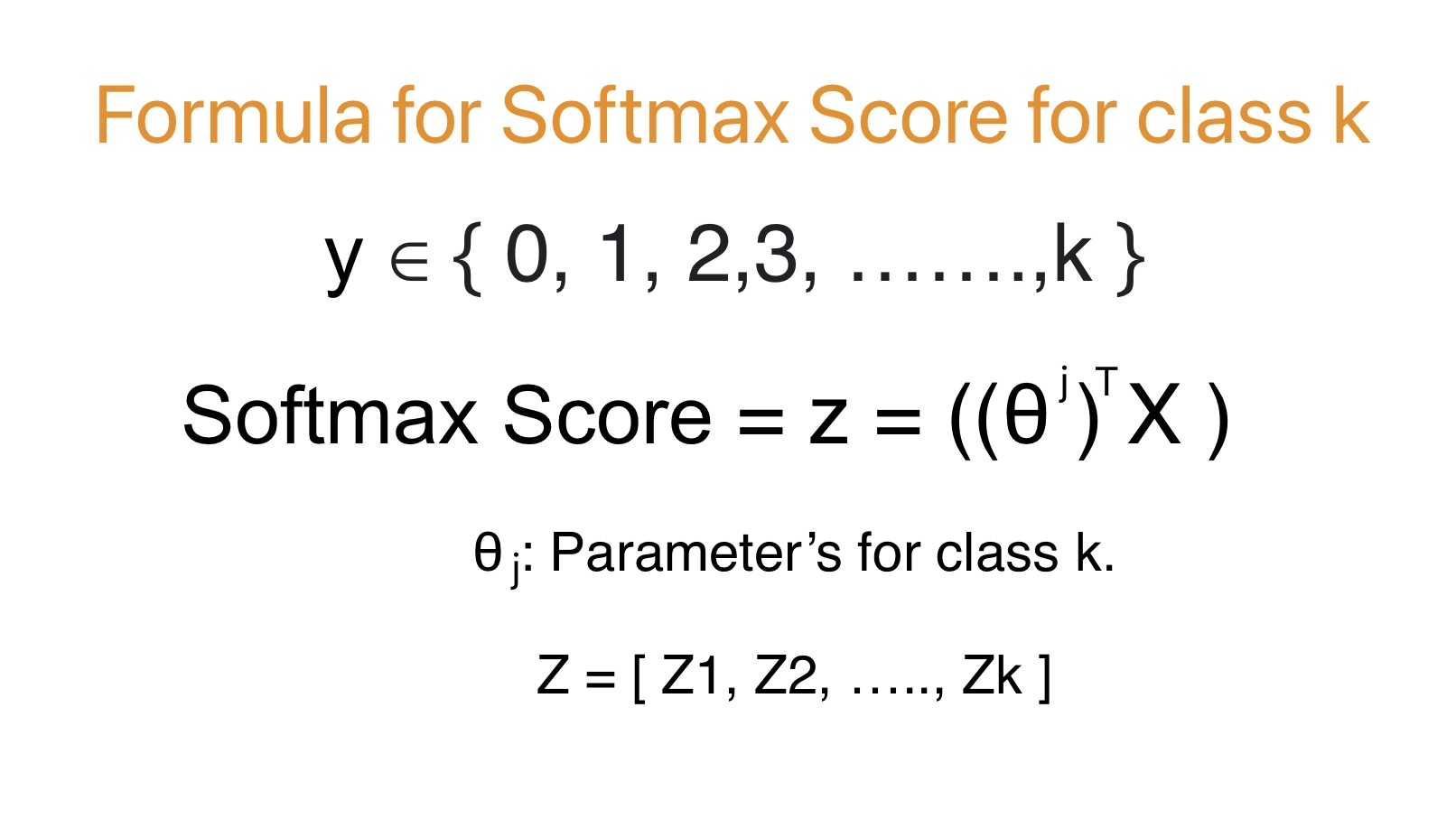
The above formula outputs an array that consist of values for softmax score for class k. We will use softmax score as an input to softmax function to calculate the probability of an instance belonging to a class k.
Softmax Function
The softmax function is a mathematical function that takes a vector of numerical scores as input and transforms them into a probability distribution over multiple classes. We can use for as an output layer of a neural network for multi-class classification problems and Softmax Regression.
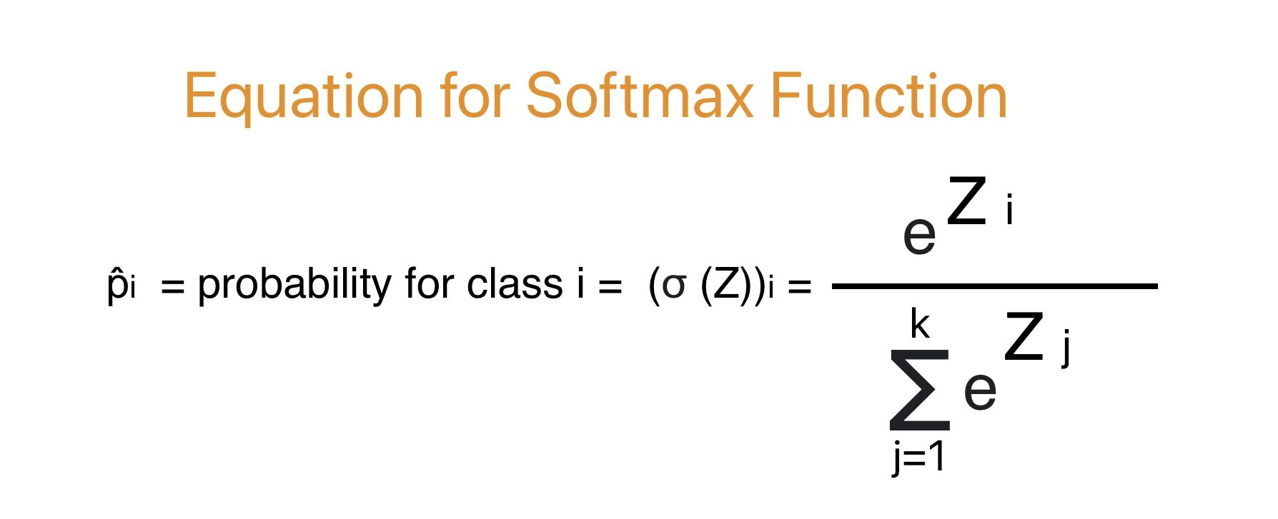
- The above function outputs the probability of each class where the total probability is equal to 1.
- It amplifies the probabilities of larger input values while reducing for smaller values. In other words, the softmax function gives a high probability the the highest raw score and decrease the values exponentially where the score deviates from the maximum.
Argmax Function
For any unknown instances we need to calculate probability for each class and give this input to argmax function.
The argmax operator returns the value of a variable that maximizes a function.
Cost function for Softmax Regression in Machine Learning
The cost function for softmax regression model is also known as cross entropy function. This function penalizes the classification model when it estimates a low probability for the target or actual class.
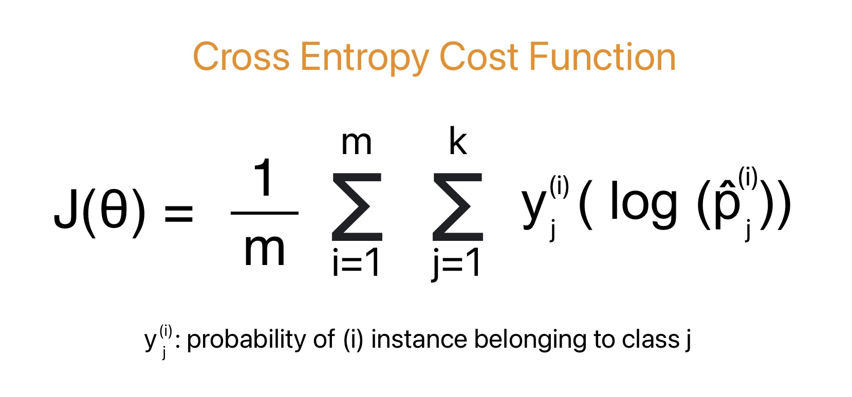
We can conclude the following points from the formula of the cross entropy function:
- Its value varies from O to 1.
- It gives the target probability of an instance belonging to a given class.
- If several classes are equal to two; The cost function becomes equivalent to the logistic regression cost function.
Gradient vector for Cost Function / Cross Entropy Function
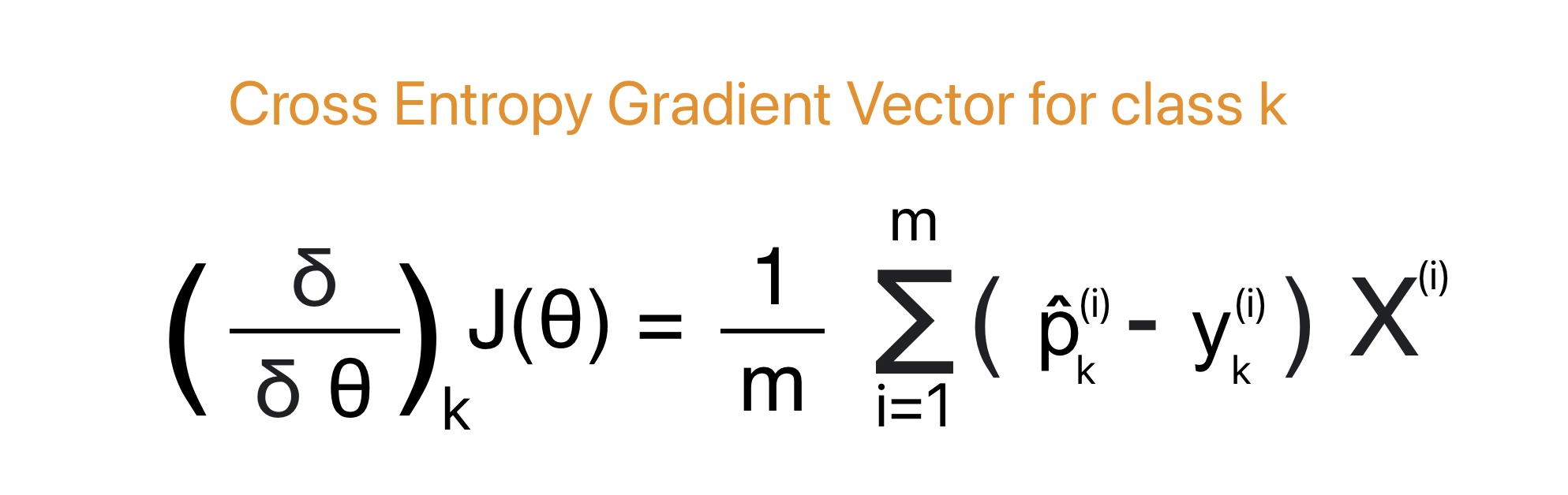
We can use Gradient Descent in softmax regression to find the weight matrix that minimizes the cost function.
Implementation of Softmax Regression in Python
We will use Softmax Regression to classify the iris flowers into all three classes. Scikit-Learn’s LogisticRegression uses one-versus-all by default when we train it on more than two classes. For softmax regression, we can set the multi_class hyperparameter to “multinomial”.
We can use “lbfgs” solver for softmax Regression. It applies ℓ2 regularization by default, which we can control using the hyperparameter C.
Training and Predicting Values using softmax regression
# Import Required Library
from sklearn.datasets import load_iris
from sklearn.model_selection import train_test_split
from sklearn.preprocessing import StandardScaler
from sklearn.linear_model import LogisticRegression
from sklearn.metrics import accuracy_score, classification_report
import numpy as np
Data Preparation
# Load the Iris dataset for multi-class classification
iris = load_iris()
Next step is to understand your data similar to the way we did in the article on logistic regression. We will not cover this here.
# For understanding purpose we will condider two feature petal length, petal width
X = iris.data[:, (2, 3)]
y = iris.target

# Split the data into training and testing sets
X_train, X_test, y_train, y_test = train_test_split(X, y, test_size=0.2, random_state=26)
# Standardize the features
scaler = StandardScaler()
X_train = scaler.fit_transform(X_train)
X_test = scaler.transform(X_test)Create Softmax Regression model
# Create and train the softmax regression model
softmax_model = LogisticRegression(multi_class='multinomial', solver='lbfgs', random_state=42)

# Create and train the softmax regression model with regularization
#softmax_model = LogisticRegression(multi_class='multinomial', solver='lbfgs',C = 10, random_state=42)

softmax_model.fit(X_train, y_train)
# Make predictions on the test set
y_pred = softmax_model.predict(X_test)# Evaluate the softmax regression model
accuracy = accuracy_score(y_test, y_pred)
print(f"Accuracy: {accuracy:.2f}")# Display classification report
print("Classification Report:")
print(classification_report(y_test, y_pred))Predicting Values
# Predictions of unknown instance class
softmax_model.predict([[2, 3]])
# Prediction of probability of unknown instance
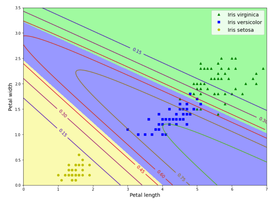
softmax_model.predict_proba([[2, 3]])Decision Boundary for Softmax Regression
We will use the above trained softmax regression model to plot the decision boundary.
# Create a mesh grid
x0, x1 = np.meshgrid(np.linspace(0, 8, 500).reshape(-1, 1), np.linspace(0, 3.5, 500).reshape(-1,1))
# Crete a new flat matrix
X_new = np.c_[x0.ravel(), x1.ravel()]
X_new.shape# Standardize the new points using scaler we used during training of data
X_new_standardized = scaler.transform(X_new)# Calculate the probability of each element
y_proba = softmax_model.predict_proba(X_new_standardized) # Values in y_proba will vary from 0 to 1
# This will list the probabilities of second type of flower 'versicolor' at index 1
y_proba_versicolor = y_proba[:, 1].reshape(x0.shape) #Predict the class for unknown Values
y_predict = softmax_model.predict(X_new_standardized)
y_predict_allflower = y_predict.reshape(x0.shape)Plot the Decision Boundary
# Import Required library to plot the decision boundary
import matplotlib.pyplot as plt
from matplotlib.colors import ListedColormap
plt.figure(figsize=(12, 9))
# Plot data between length vs width if flower is virginica
plt.plot(X[y==2, 0], X[y==2, 1], "g^", label="Iris virginica")
# Plot data between length vs width if flower is versicolor
plt.plot(X[y==1, 0], X[y==1, 1], "bs", label="Iris versicolor")
# Plot data between length vs width if flower is setosa
plt.plot(X[y==0, 0], X[y==0, 1], "yo", label="Iris setosa")
# Define the colormap
custom_cmap = ListedColormap(['#fafab0','#9898ff','#a0faa0'])
# This will add the shaded area
plt.contourf(x0, x1, y_predict_allflower, cmap=custom_cmap)
contour = plt.contour(x0, x1, y_proba_versicolor, cmap=plt.cm.brg)
# Add labels to the graph
plt.clabel(contour, inline=1, fontsize=12)
plt.xlabel("Petal length", fontsize=14)
plt.ylabel("Petal width", fontsize=14)
plt.legend(loc="upper right", fontsize=14)
plt.axis([0, 7, 0, 3.5])