We discussed in our previous article on linear regression that we can use regression analysis to solve classification problems. This article is a beginner’s guide to Logistic Regression in Machine Learning.
Table of Contents
ToggleWhat is Logistic Regression?
Logistic Regression in machine learning is a binary classifier (Positive/1 or Negative/0 class) that estimates the probability of an instance belonging to a given class.
The logistic regression model predicts the instance belonging to a positive class if its probability is greater than 50%. For example, we can use logistic regression to determine the probability of email being spam.
Logistic regression assumes a linear relationship between the features and the log-odds of the response variable.
Advantages of Logistic Regression in Machine Learning
Logistic regression is a widely used machine-learning technique for binary classification. Here is the list of advantages of logistic regression in machine learning.
- It is similar to understand and works similar to linear regression to some extent.
- Along with binary classification, logistic regression gives the output probability of a decision as well. For example, if you are using logistic regression for spam classification. It can output like there is a 67% probability that this email is spam.
- Logistic Regression tends to have lower variance compared to other algorithms.
- It does not assume a linear relation between the two features.
- We can use L1 and L2 regularization in linear regression to prevent overfitting.
Limitations of Logistic Regression in Machine Learning
Along with the above advantages, logistic regression has the following limitations as well.
- Best used for binary classification only.
- Logistic regression creates a linear decision boundary. Therefore it can separate two classes linearly only.
- Works best while dealing with a relatively small dataset.
Application examples of Logistic Regression in Machine Learning
Logistic regression in machine learning is one of the versatile algorithm that has application in various fields to solve binary classification problems.
It’s important to note that we can also use logistic regression in machine learing to handle multiclass classification problems using techniques like one-vs-rest or one-vs-one. But it has very limited applications due to complexity involved. Here is the list of application examples of logistic regression in machine learning.
In Manufacturing Industry
In manufacturing industry or production line we can use logistic regression to predict if a product will meet all the required quality parameters according to output from few features.
Medical
Based on a person full body checkup results such sugar level, blood pressure cholesterol etc. Logistic regression machine learning algorithm can determine the probability of a person having a heart problem.
Customer Churn
Logistic regression analysis is used to determine the list of customers that can churn. Marketing team can use this analysis to make contacts with right customers and retain them.
Sentiment Analysis
Logistic regression can be used to classify text as positive or negative sentiment. This works as an input to other machine learning algorithms.
Fraud Detection
Logistic regression is used by banks to detect fraudulent activities.
E- Commerce
Based on a person activities e-commerce companies can determine whether a person will purchase a product or not.
How Logistic Regression Works?
Like linear regression, Logistic regression also computes the weighted sum of input features & the bias term and outputs the results in logistic form (0 or 1) instead of continuous data. Logistic regression in machine learning uses a logistic function (e.g. Sigmoid Function) to convert continuous data into logistic form.
Prior Conditions for Logistic Regression in Machine Learning
Here is the list of prior conditions or assumptions of the logistic regression in the machine learning model. We need to ensure these assumptions are fulfilled before implementing logistic regression in machine learning.
Linear Relation
Linear Relationship between independent variables or features and the dependent variable. The model may not perform well if the relationship is not linear.
Binary Outcome for Dependent Variable
For binary logistic regression, the dependent variable should have two categories only. You need to use softmax regression or the One vs all technique if the dependent variable has more than two categories.
Independent Observations
This assumption for logistic regression ensures the values of independent variables are not influenced by the dependent variables.
Absence of Multicollinearity
Multi-collinearity occurs in data when two or more independent variables are correlated. Logistic regression in machine learning assumes that Multi-collinearity does not exist in data.
Absence of Outliners
Logistic regression in machine learning is very sensitive to outlines. They can impact the values for selected parameters.
The scale of Independent Variables
It is not mandatory but a good practice to ensure the independent variables are on the same scale for logistic regression.
Decision Boundary for Logistic Regression
The Goal of Logistic Regression is to find a best fit line or a decision boundary that separates the two classes.
The decision boundary in logistic regression is a hyperplane that separates the feature space into binary classes using a line. This decision boundary line can be linear or polynomial.
The decision boundary is nothing but just a equation of a line or hyperplane.
Equation for Logistic Regression
The equation of logistic regression is a sigmoid function where the variable is the equation of line. This function will give output between 0 to 1 and it gives probability of a variable belonging to positive class.
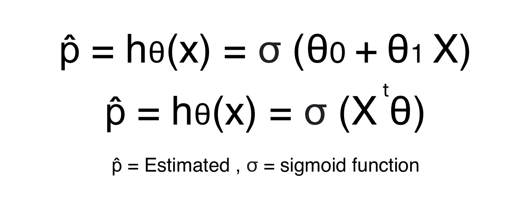
The goal of logistic regression in machine learning is to determine the parameters or weights that gives high probabilities for positive instances and low probability for negative instances.
For unknown instance, we calculate the value of y for given X. We declare a instance positive if the calculated y or probability is greater than 0.5 or 50%.
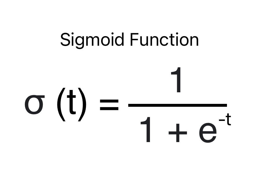
What is Sigmoid Function?
The sigmoid function is an s-shaped function that outputs a number between 0 and 1.
Cost Function for Logistic Regression in Machine Learning
The cost function is also known as loss function. The goal of cost function in logistic regression is penalize the ML model if the prediction is not correct. Therefore we derive the Cost function for logistic regression from the likelihood function.
Likelihood Function
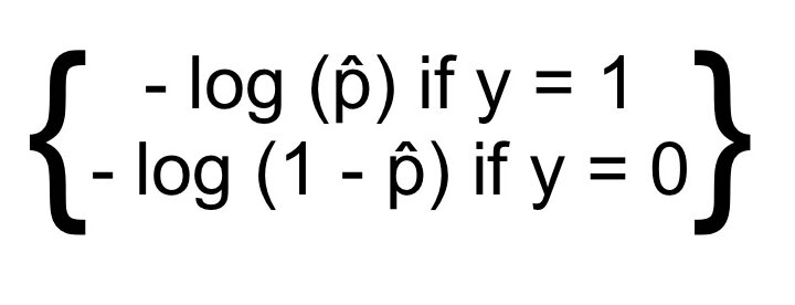
Log ( p̂) in above likelihood function becomes very large when p̂ approaches 0.
- The cost will be high if the model predicts a probability close to 0 for a positive instance.
- Error will also be high if the logistic regression model predicts a negative class as positive.
Formula for Cost Function
Now we will drive cost function from above likelihood function. For a binary classification problem, where the target variable y is either 0 or 1, the logistic regression cost function J(θ) for parameters θ is given by:
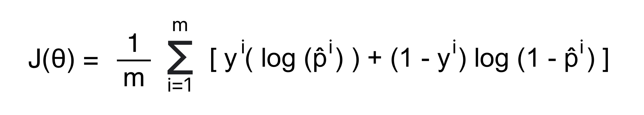
The goal of training the logistic regression algorithm in machine learning is to find weights or parameters that minimize the cost function. The above cost function is convex in shape. Therefore, we can use gradient descent to find the global minima and calculate the parameters that minimize the cost function.
Partial Derivative for cost function
We calculate partial derivatives of the cost function for each parameter to update the weight (θ) using gradient descent. The partial derivative of the logistic regression cost function for the j parameter (θj) is given by:
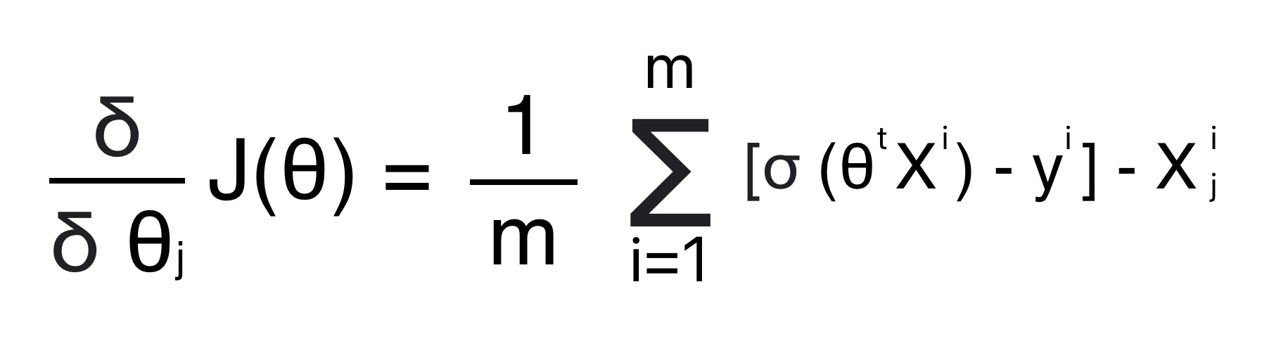
m: Number of training examples.
σ(θ(j) X(i)) : Sigmoid function applied to the linear combination of features
y (i)
: Actual label (0 or 1) for i th training example.
X
j
(i) : jth feature of the
ith training example.
The partial derivative of the cost function gives the rate of change of the cost function for the jth parameter. During the gradient descent optimization process, the parameters are updated using the following formula:
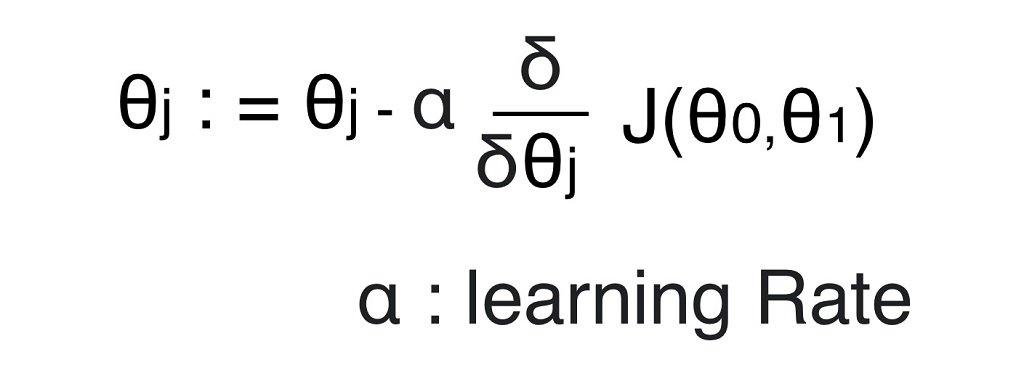
We can use the above equation iteratively to find the optimal values for the parameters θ that minimize the logistic regression cost function. The process continues until convergence is achieved or a predefined number of iterations is reached.
Implementation of Logistic Regression in Python
We will use the Breast Cancer Wisconsin dataset available in scikit-learn. In this example, we will perform binary classification to predict whether a breast cancer tumor is malignant or benign.
# Import required libraries
import numpy as np
import matplotlib.pyplot as plt
from sklearn import datasets
from sklearn.model_selection import train_test_split
from sklearn.preprocessing import StandardScaler
from sklearn.linear_model import LogisticRegression
from sklearn.metrics import accuracy_score
# Load the Breast Cancer Wisconsin dataset
cancer = datasets.load_breast_cancer()# There are multiple features but for sake of understanding we will use two features only
X = cancer.data[:, :2] # Crete input features
y = cancer.target # 0 for malignant, 1 for benign type of cancer# Split the dataset into training and testing sets
X_train, X_test, y_train, y_test = train_test_split(X, y, test_size=0.2, random_state=42)# Standardize the features
scaler = StandardScaler()
X_train = scaler.fit_transform(X_train)
X_test = scaler.transform(X_test)# Create and train the logistic regression model
lr_model = LogisticRegression(random_state=42)
lr_model.fit(X_train, y_train)# Make predictions on the test set
y_pred = lr_model.predict(X_test)# ML Model Evaluation using accuracy
accuracy = accuracy_score(y_test, y_pred)
print("The prediction model accuracy in test data is:",accuracy)The prediction model accuracy in test data is: 0.9035
We suggest you read this article to understand more on Machine learning model evaluation techniques.
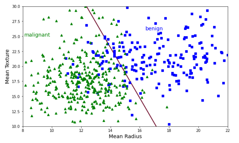
Logistic Regression Decision Boundary with two Features
The first step in creating the decision boundary is to create a mesh grid for input features.
- Mesh-Grid turns one-dimensional NumPy arrays into grids called matrices.
- We get two matrices back if we pass two NumPy arrays into the mesh grid.
- Mesh-grid takes two arrays of different lengths and manipulates them.
- The first feature values are arranged in rows whereas the second feature values are arranged in columns.
- In the first matrix, every column has a different number. In the second matrix, every row has a different number.
# Get the minimum and maximum value in feature 1 and feature 2 respectively
x0_min, x0_max = X[:, 0].min() - 1, X[:, 0].max() + 1
x1_min, x1_max = X[:, 1].min() - 1, X[:, 1].max() + 1
x0, x1 = np.meshgrid(np.linspace(x0_min, x0_max, 500).reshape(-1, 1), np.linspace(x1_min, x1_max, 500).reshape(-1,1))
The next step is to flatten the meshgrid array and create new matrix that we will use to create the decision boundary.
# x0.raval will out a continuous array. for example, a 2X3 array will become 6 x 1 array
# np.c_ : Concate two metrics into an array
X_new = np.c_[x0.ravel(), x1.ravel()]
# Standardize the new points using the same scaler
X_new_standardized = scaler.transform(X_new)# Calculate the probability of each element
y_proba = lr_model.predict_proba(X_new_standardized) # Values in y_proba will vary from 0 to 1
#predict_proba will output two column
# the first column will represent the probability of instance belonging to negative class (0)
# the second column will represent the probability of instance belonging to positive class (0)
y_proba_positive = y_proba[:, 1].reshape(x0.shape) # this will give the probability of positive output# Plot the decision boundary and data points
plt.figure(figsize=(10, 6))
plt.contour(x0, x1, y_proba_positive, levels=[0.5], cmap="RdBu", linewidths=2)
plt.plot(X[y==0, 0], X[y==0,1], "bs")
plt.plot(X[y==1, 0], X[y==1, 1], "g^")
plt.clabel(contour, inline=1, fontsize=12)
plt.text(9, 25, "malignant", fontsize=14, color="g", ha="center")
plt.text(17, 26, "benign", fontsize=14, color="b", ha="center")
plt.xlabel("Mean Radius", fontsize=14)
plt.ylabel("Mean Texture", fontsize=14)
plt.axis([8, 22, 10, 30])