The best practice to implement an ML algorithm is to understand how it works mathematically. It will help in selecting the right hyper-parameters as per requirements. Linear regression algorithm in ML is one of the simplest Machine Learning algorithms where dependent and independent variables are linearly related.
Regression is a statistical technique to establish a relationship between the dependent (y) and multiple independent (X) variables. This relationship can be linear, parabolic, or something else in nature. Linear Regression is a part of regression techniques.
Table of Contents
ToggleWhat is Linear Regression Algorithm in ML?
Linear Regression is a statistical technique to determine a Linear Relation between Independent and multiple dependent variables. This relationship can be linear, parabolic, or something else in nature.
The ultimate goal of running LR analysis is determining parameters that create a straight line with minimum error.
Let’s consider this dataset where X is independent, and y is the dependent variable. This is a supervised machine learning problem because the output/ dependent variable is known.
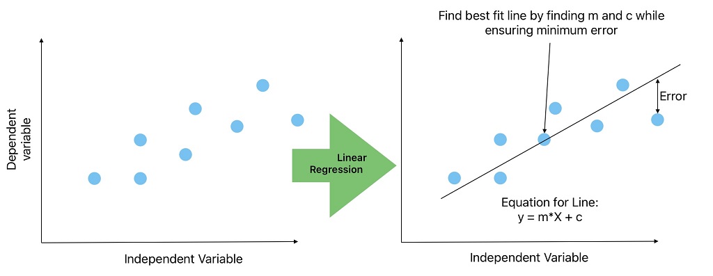
The first step in ML problem-solving is to visualize the data. When we plot a graph between the independent (X) and dependent (y) variables and find the relationship is linear. We become confident in solving this problem using a simple linear regression algorithm.
In a simple linear regression algorithm, we will find the best line that ensures a minimum error (Root Sum of Square Error, Root Mean Square Error) in all training data. Afterward, we can predict the unknown y values for given values of X from the best-fit line.
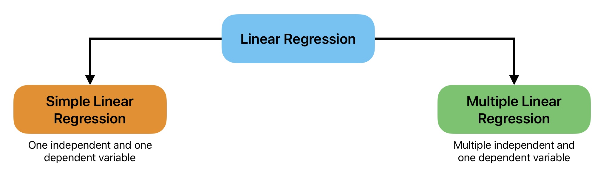
We can classify linear regression models in machine learning into the following two types according to the number of independent variables.
- Simple Linear Regression
- Multiple Linear Regression
Simple Linear Regression Algorithm in Machine Learning
A Simple Linear Regression Model is a type of linear regression with one independent variable. This model is quite simple to visualize and solve with minimum complexity.
Equation
y = m X + C
y = b0 + b1 X
hθ(x) = θ0 + θ1 X
Where:
y = Dependent Variable;
X= Independent Variable;
b0 and b1 or θ0 and θ1 are linerar Regression model parameters or weights.
Multiple Linear Regression Algorithm
A Multiple Linear Regression Algorithm is a type of linear regression with multiple independent and one dependent variable. It becomes very difficult to visualize multiple linear regression model as we increase number of variables.
Equation
y = θ0 + θ1 X1 + θ2 X2 +.....+ θn Xn
Where:
y = dependent variable;
X1, X2,..., Xn are independent variables;
θ0, θ1, θ2,......, θn are n multiple linear regression parameters;
Here the goal of the multiple linear regression algorithm is to calculate the parameters that minimize the squared error. A Linear regression model makes a prediction by calculating the sum of weighted average of the input features and a constant.
Vector form of Linear Regression Model
y = X.θ
Where:
y = A column vector of the dependent variable.
X = Input features or independent variable matrix. The values in the first column of this matrix are ones.
θ = A column vector for coefficients
We can write the above equation in the following matrix form:
Common Challenges in Linear Regression Model Development
It is comparatively easy to develop linear regression algorithms. However, we face many challenges to ensure the quality linear regression algorithm. Here is the list of common challenges during linear regression algorithm development.
- Outliners in data impact linear regression parameters. As a result, the LR model does not perform as expected on training and test data.
- Overfitting is a problem when the ML model performs better on training data and does not generalize on unseen test data.
- Underfitting is a common problem in LR models. It occurs when the algorithm performs poorly on training and test data.
- Any violation in Linear regression prior conditions leads to inefficient weight estimation.
- Correlation in independent variables leads to wrong parameter estimation because linear regression considers the impact of independent variable additive.
- Inappropriate selection of parameters may lead the solution to local minima.
How to implement Linear Regression ML Algorithm?
We can use the following two approaches to solve linear regression problems in ML.
- Direct Approach: Directly compute the model parameters that minimize the cost function on training data.
- Gradient Decent: Iterative optimization approach that minimizes the cost function on training data.
Both of the above approaches to minimizing the cost function and selecting the best parameters have their advantages and limitations.
Here is the list of prior conditions or assumptions of the linear regression machine learning model. We need to ensure these assumptions are fulfilled before implementing linear regression.
- Linear Relationship between independent and dependent variable.
- Multi-collinearity does not exist in data.
- No Auto-correlation exists.
- Homoscedasticity.
- Normally Distributed Prediction Error.
Cost Function for Linear Regression Algorithm
Our Goal during Linear Regression model development is to find the parameters that minimize the Root Mean Squared Error (RMSE) or Mean Squared Error (MSE). It is comparatively easy to minimize MSE compared to RMSE. But both functions give similar results.
The cost function also known as the loss function is mean squared error for linear regression algorithm. In other words, cost function is error that we want to minimize on training data.
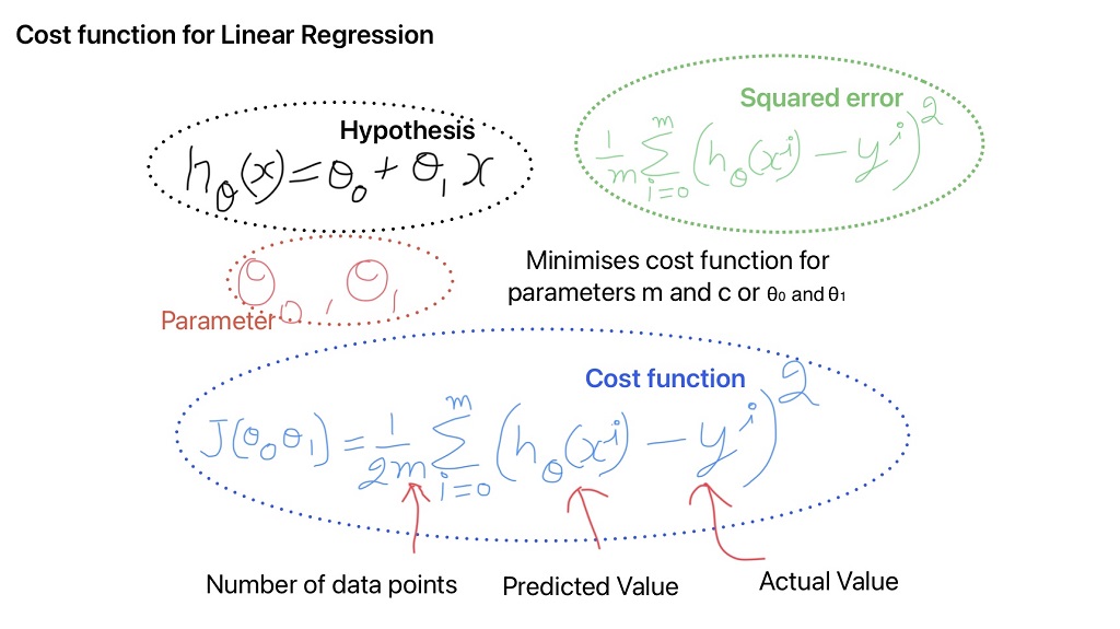
Why cost function is divided by "2m"
The cost function is divided with 2m instead of m, just to simplify the calculations when calculating the derivative or minimizing the cost function.
Direct Approach to Solve Linear Regression Problems
We can use one of the following two approaches to calculate the unknown coefficient.
- Normal Equation Approach
- Singular Value Decomposition (SVD) Approach
Normal Equation Approach to determine unknown coefficients
θ = (XTX)-1 X T y
Here θ is a vector of unknown coefficients that minimizes the cost function. Now we will use python code to determine unknown coefficients using normal equation.
Python Code to solve Normal Equation for Linear Regression Model Development
The Normal Equation computes (n + 1) × (n + 1) matrix (where n is the number of features) to solve the linear regression problem. If we double the number of features, the computation time increases drastically.
# Import Required Library
import numpy as np
import pandas as pd
import matplotlib.pyplot as plt

%matplotlib inline
import matplotlib as mpl
We will use the NumPy library to generate the training data. Afterward, we will plot this data using the Matplot library.
# Generate Dependendent and Independent values considering equation y = 5*X + 6 + error (y = mX+c+error)
X = 1.5 * np.random.rand(100, 1) #Generate a random data with uniform distribution
# Generates a NumPy array with shape (100, 1) filled with random values (mean=0, standard deviation=1).
error = np.random.randn(100, 1)
y = 5 * X + 6 + error
# Plotting the X and y data
plt.plot (X, y, "b.")
plt.xlabel("$x_1$", fontsize=18)
plt.ylabel("$y$", rotation=0, fontsize=18)
plt.axis([0, 1.5, 2, 16]) # limit the graph size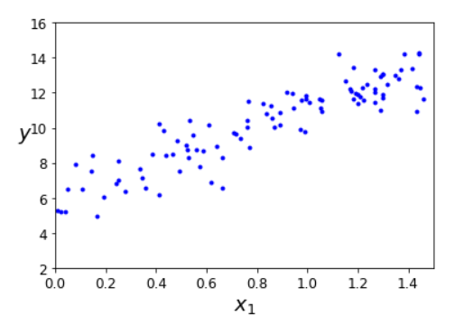
Just by looking at the above image, we can say that a straight line can fit the input data. Therefore we can use simple linear regression here.
The next step to solve normal equations to develop a linear regression model is to add a column to independent data.
X_b = np.c_[np.ones((100, 1)), X]

# np.ones((100, 1)) will create a 100 X 1 matrix with all exlements = 1)
# np.c_ function will join two matrices by column
# np.c_[100X1_matrix, 100X1_matrix] : Output will be a 100 X 2 matrix the first columns will be all 1

print(X_b.shape)
# Implementing the normal equation to calculate coefficients
coeff_best = np.linalg.inv(X_b.T.dot(X_b)).dot(X_b.T).dot(y)
# X_b.T : Calculates the transpose of the matrix
# (X_b.T).dot(X_b) : Calculates the dot product of (X_b.T) and (X_b)
# np.linalg.inv(matrix): Calculate the inverse of matrix
print("Best Coefficient values are:",coeff_best )Best Coefficient values are: [[6.22343373] [1.69388673]]
The calculated coeff_0 and coeff_1 are 6.223 and 1.69388 respectively. But in our initial equation “y = 6 + 2 * X + error” we considered this as 6 and 2 respectively. Therefore calculated values are closer to actual values.
# Predicting unknown values of x
X_new = np.array([[0], [2]])
X_new_b = np.c_[np.ones((2, 1)), X_new] # This will add x0 = 1 to each instance
y_predict = X_new_b.dot(coeff_best) # dot product of X with X0 and theta_best
print("Predicted values for Y for x_new are:", y_predict)
Predicted values for Y for x_new are: [[6.22343373] [9.61120718]]
# Plotting the Best Fit Line
plt.plot(X_new, y_predict, "r-") # This will plot a line for x and y
plt.plot(X, y, "b.") #This will plot the predicted points for X and y respectively
plt.axis([0, 1.5, 3.5, 10])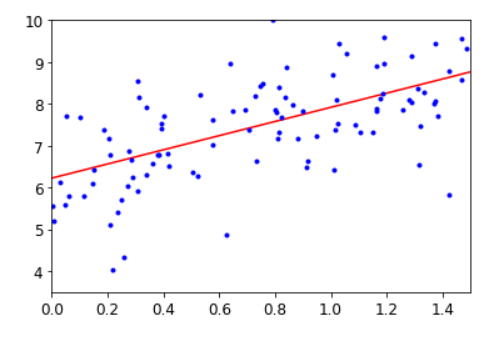
Singular Value Decomposition (SVD) Approach for Linear Regression
In the SVD approach, we calculate linear regression model coefficients using Scikit-Learn’s LinearRegression class.
- SciPy library calculates the pseudo-inverse using a standard matrix factorization technique Known as Singular Value Decomposition (SVD). SVD decomposes the training set matrix X into the matrix multiplication of three matrices.
- A normal Equation does not work if the dot product of the matrix transpose of X and X is not singular. In such cases, pseudo-inverse is the best approach to solve machine learning problems.
- If we double the number of features, the computation time will be 4 times in SVD.
SVD Implementation example in Python for Linear Regression Model Development
# Import the sklearn LinearRegression Library
from sklearn.linear_model import LinearRegression
# Call Linear Regression function
lin_reg = LinearRegression()
# Train Linear Regression model on Previous Data.
#There is no need to change the add column in independent variable data
lin_reg.fit(X, y)
# Getting Coefficient Values from Trained Linear Regression Model
print("Best Coefficient values are:", lin_reg.intercept_, "and", lin_reg.coef_)Best Coefficient values are: [6.22343373] and [[1.69388673]]
The output values are similar to values we calculated from normal equation method.
Limitations of Solving Linear Regression Problem using Direct Method
- The normal Equation approach to finding the unknown parameters is computationally expensive. If we double the number of features, the computation requirements increase 8 times.
- The SVM approach is comparatively less expensive than the normal equation approach. If we double the number of features the computation requirements will increase 4 times.
- Both the normal equation and SVM approaches are best used when the number of features is relatively less.
We can also use a gradient descent approach to determine unknown parameters. It is an alternative approach to the direct method and comparatively less computationally expensive. We can use this approach if the number of features is relatively large.
To implement gradient descent all features must be on the same scale. The applications of gradient descent are not only limited to linear regression algorithm.
Inputs for Gradient Decent
We need the following inputs to implement gradient descent to determine the unknown parameters that minimize the cost function.
- Random initialization values for parameters (theta).
- Learning Rate
- Maximum Number of Iterations
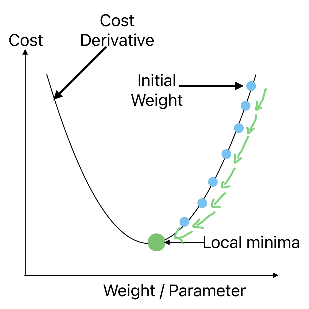
How MSE Cost Function Handles Irregular Cost Function Problem
The following two points ensure gradient descent reaches a global minimum provided the number of iterations is enough and the Learning rate is not large.
- The MSE cost function for a Linear Regression is a convex function. It means that if we pick any two points on the curve, the line joining them never crosses the curve. As a result, there are no local minima, just one global minimum.
- It is also a continuous function with a slope that never changes abruptly.
Implementation of Batch Gradient Descent in Python
Define Required input for Batch Gradient Descent
eta = 0.1  # Defining the Learning Rate
n_iterations = 1000 # Defining Maximum numbner of Iterations
m=100 # Number of data points

theta = np.random.randn (2,1) # Random Initialization of theta
print("Random initialized value for theta are:", theta)
Random initialized value for theta are: [[ 0.10850119] [-0.56628056]]
Random initialized values may or may not be different.
Running Code for batch Gradient Descent
for iterations in range(n_iterations):
    gradients = (2 / m)*(X_b.T).dot(X_b.dot(theta)-y)
    theta = theta - eta * gradients
print ("The best value for theta is:", theta)
The best value for theta is: [[6.22343373] [1.69388673]]
- Above code callculates the theta for the defined number of iterations.
- The calculated theta values are similar to what we observed earlier with SVD or normal equation.
Stochastic Gradient Decent Algorithm
Instead of using all training data to calculate the gradient, Stochastic Gradient Descent uses random instances in the training data at every step. As a result, the algorithm becomes fast since it has to compute small data at every iteration.
Stochastic Gradient Descent works in the following steps:
- Pick a random instance in the training set at every step.
- Computes the gradients based only on that single instance.
- Update the weights.
Implementation of Stochastic Gradient Descent with simple learning schedule in Python
eta = 0.1  # Defining the Learning Rate
n_iterations = 1000 # Defining Maximum numbner of Iterations
m=100 # Number of data points

n_epochs = 50
# n_epochs: Number of times a learning algorithm passes through the training data
t0, t1 = 5, 50 # Learning schedule hyperparameters

# Define a function for learning schedule

def learning_schedule(t):
    return t0 / (t + t1)
theta_sgd = np.random.randn(2 , 1) # Randomization of theta
for epoch in range(n_epochs):
    for i in range(m):
        random_index = np.random.randint(m) #Generate a random number from 0 to (m-1)
        xi = X_b[random_index : random_index+1]
        yi= y[random_index : random_index+1]
        gradients = 2 * xi.T.dot(xi.dot(theta_sgd) - yi) #Calculation of gradiants
        eta = learning_schedule(epoch * m + i) #learning Rate will change wrt epoch number and sample number
        theta_sgd = theta_sgd-eta*gradients
print ("The best value for theta is:", theta_sgd)
The best value for theta is: [[6.22911403] [1.69601783]]
Implementation of SGD in Python using Scikit-Learn SGDRegressor class
We can also use Scikit-Learn SGDRegressor class to do stochastic gradient decent.
from sklearn.linear_model import SGDRegressor
sgd_reg = SGDRegressor(max_iter=1000, tol=1e-3, penalty=None, eta0=0.1)
sgd_reg.fit(X, y.ravel())
print ("The best value for theta is:", sgd_reg.intercept_, sgd_reg.coef_)
The best value for theta is: [6.1550789] [1.69565741]
- The above coefficient values are quite similar to what we calculated with the normal equation
Mini-Batch Gradient Decent Algorithm
Mini-batch Gradient Descent takes advantage of both batch GD and Stochastic GD. Mini-batch GD computes the gradients on small random sets of instances called mini-batches.
theta_path_mgd = []

n_iterations = 100
minibatch_size = 20

np.random.seed(42)

theta_mini = np.random.randn(2, 1)  # Random initialization of theta

t0, t1 = 200, 1000  # Corrected variable names
def learning_schedule(t):
    return t0 / (t + t1)

t = 0

for epoch in range(n_iterations):
    shuffled_indices = np.random.permutation(m)
    X_b_shuffled = X_b[shuffled_indices]
    y_shuffled = y[shuffled_indices]
    for i in range(0, m, minibatch_size):
        t += 1
        xi = X_b_shuffled[i: i + minibatch_size]
        yi = y_shuffled[i: i + minibatch_size]
        gradients = 2 / minibatch_size * xi.T.dot(xi.dot(theta_mini) - yi)  # Corrected variable name
        eta = learning_schedule(t)
        theta_mini = theta_mini - eta * gradients
        theta_path_mgd.append(theta_mini.copy())  # Append a copy of theta_mini to the path

print("The best value for theta with minibatch gradient descent is:", theta_mini)
The best value for theta with minibatch gradient descent is: [[6.20309696] [1.67912157]]
Comparison of Linear Regression Algorithms
| Algorithm | Number of training Samples | Number of Features | Scaling Required | Scikit-learn Library |
|---|---|---|---|---|
| Normal Equation | Does't Matter | Best for Small number of features | No | NA |
| SVD | Linear Regression | |||
| Batch GD | Small | Does't Matter | Yes | SGDRegressor |
| Stochastic GD | Does't Matter | |||
| Mini Batch GD |
How can we improve the accuracy of Linear Regression Model?
We can improve linear regression model accuracy by ensuring the quality of training data and selecting the right hyperparameters. Here is the list of points we can consider to improve the ML model accuracy.
Handling the Outliners
Outliners can greatly impact the performance of machine learning algorithms. According to your data and requirements, you can decide on whether you want to remove the outliner or replace the outliner with some other data.
Handling the Missing values
Missing values in data impact the linear regression model performance. Some missing values are important and data engineers need to decide on how to handle missing values so that it has minimal impact on model performance.
Feature Selection
Best machine learning algorithms have only relevant features. Therefore the best practice is to remove irrelevant or redundant features that do not have a significant impact on parameter selection.
Regularization Techniques
We can use one of the following regularization techniques to improve the machine learning model performance.
- Ridge Regression
- Lasso Regression
- Early Stopping
Independent Variable Scaling
We need to scale the input features if we are using gradient descent techniques to select the best parameters.
Hyper Parameter Tuning
We can use grid search, randomized search, or cross-validation techniques to select the best parameters for linear regression.
Frequently Asked Questions on Linear Regression
Linear Regression is a statistical technique to determine a Linear Relation between Independent and multiple dependent variables. This relationship can be linear, parabolic, or something else in nature.
Regression line is also known as best fit line is a straight line that defines a relationship between dependent and independent variables.
No, its a regression algorithm to determine the continuous variables.
We can use one of the following techniques to calculate the error in linear regression.
- Mean Square error
- Root mean square error
- Mean absolute error.
The cost function is divided with 2m instead of m, just to simplify the calculations when calculating the derivative or minimizing the cost function.
- Linear Relationship between independent and dependent variable.
- Multi-collinearity does not exist in data.
- No Auto-correlation exists.
- Homoscedasticity.
- Normally Distributed Prediction Error.
It is comparatively easy to minimize MSE compared to RMSE. But both functions give similar results.