Learning Curve in Machine Learning

Learning Curve in Machine learning is a tool to diagnose an ML model to determine the impact of new training instances on training and validation errors. It is also known as the error curve, experience curve, improvement curve, or generalization curve.

Table of Contents

What is the Learning Curve in Machine Learning

The learning curve in machine learning is a plot between the error function and the number of training instances for training and validation instances.
We can generate the learning curves by training the machine learning model several times on different sized subsets of the training set.

Learning Curves in machine learning has the following applications:

Determine the capability of the ML model to learn incrementally from the dataset.
Determine if the Machine learning model is overfitting or underfitting the training data.
To make decisions on bias-variance tradeoffs.
Determine if training and validation data are representative.
Compare different algorithms.
Improve ML model convergence.

Learning Curve for Machine Learning in Python

We will develop a function to plot learning plots in machine learning for a machine learning model using Sklearn library in python.

# Import Required Library
from sklearn.metrics import mean_squared_error
from sklearn.model_selection import train_test_split
import matplotlib.pyplot as plt

def plot_learning_curves (model, X, y, title="Learning Curve"):
    # Split Training and test data in 1:4
    X_train, X_val, y_train, y_val = train_test_split(X, y, test_size=0.2)
    train_errors, val_errors = [], []
    for m in range(1, len(X_train)):
        model.fit(X_train[: m], y_train[:m])
        y_train_predict = model.predict(X_train[:m])
        y_val_predict = model.predict(X_val)
        train_errors.append(mean_squared_error(y_train[:m], y_train_predict))
        val_errors.append(mean_squared_error(y_val, y_val_predict))
        
    #Plotting Learning Curve
    plt.figure(figsize=(8, 5))
    plt.plot(np.sqrt(train_errors), "r-+", linewidth=2, label="Training Data")
    plt.plot(np.sqrt(val_errors), "b-", linewidth=3, label="Validation Data")
    plt.title(title)
    
    plt.legend(loc="upper right", fontsize=14)
    plt.xlabel("Training set size", fontsize=14)
    plt.ylabel("Root Mean Square Error", fontsize=14)

Now we will use the above function to plot the learning curve on sample linear data using linear regression.

# Import Required Library
import numpy as np

# Generate non-linear data with noise
m = 100 # Number of training examples
X = 7 * np.random.rand(m, 1) - 4
y = 2*X + 4 + np.random.randn(m, 1)

# Import Linear Regression Library
from sklearn.linear_model import LinearRegression

lr = LinearRegression()
plot_learning_curves(lr, X, y)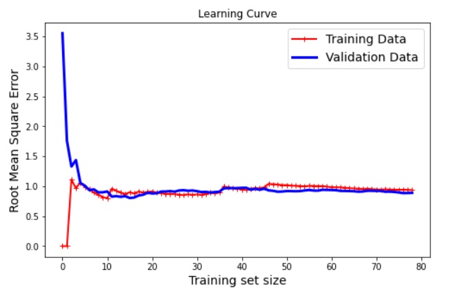

Interpretation of the Learning Curve in Machine Learning

We can make following interpretations using above learning curve in machine learning.

The machine learning model fits perfectly (low error on training data) for smaller training examples. But validation error is high at the same time.
If we increase the training data, training error increases whereas, validation error starts decreasing. In other words machine learning model stats generalizing.
After a certain limit both training and validation error becomes constant.

Example of Learning Curve that detects Overfitting

Now, we will create a second degree of polynomial data and will try to fit this data using 10 degree of polynomial. This will generate a overfitting issue in Machine Learning. Now we will try to detect this issue using learning curve.

# Generate non-linear data with noise
X_2 = 7 * np.random.rand(20, 1) - 1
y_2 = 2 * X_2**2 + 0.5*X_2 + 4 + np.random.randn(20, 1)

# Import Linear Regression Library
from sklearn.linear_model import LinearRegression 
from sklearn.preprocessing import PolynomialFeatures
from sklearn.pipeline import Pipeline

# Define pipeline for Polynomial Regression
polynomial_regression = Pipeline([("poly_feature", PolynomialFeatures(degree=10, include_bias=False)), 
                                ("lr", LinearRegression())])

# Plotting the Learning Curve
plot_learning_curves(polynomial_regression, X_2, y_2, "Learning Curve indicating overfit Issue")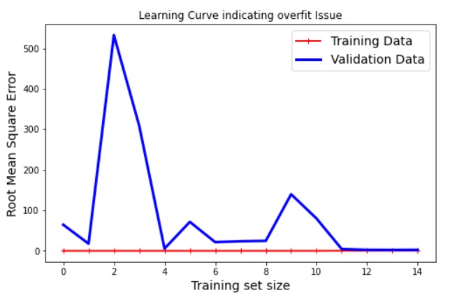

The above image indicates the machine learning model is giving high error in validation data and zero RMSE in training. This indicates overfitting issue in machine learning model.

Example of Learning Curve that indicates Underfitting

Now, we will create a third degree of polynomial data and will try to fit this data using one degree of polynomial. This will generate a underfitting issue in Machine Learning. Now we will try to detect this issue using learning curve.

# Generate non-linear data with with 3 degree polynomial and noise
X_3 = 7 * np.random.rand(20, 1) - 1
y_3 = X_3**3 + 2 * X_3**2 + 0.5*X_3 + 4 + np.random.randn(20, 1)

# Define pipeline for Polynomial Regression
polynomial_regression = Pipeline([("poly_feature", PolynomialFeatures(degree=1, include_bias=False)), 
                                ("lr", LinearRegression())])

# Plotting the Learning Curve
plot_learning_curves(polynomial_regression, X_2, y_2, "Learning Curve Indicating Underfit Issue")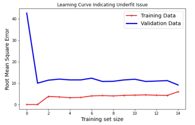

The above image indicates the machine learning model is giving high error in both training and validation data. This indicates underfitting issue in machine learning model.

“Feel free to download and explore the reference code for the learning curve in machine learning from my GitHub repository here. Happy coding!”